I am currently using a lot more the Pandas library to load data into a fuzzy learning framework. This note summarizes my learning points on the library. For the process of this exercise the Wine Quality data set used by Cortes et all will be used
Pandas Terminology
Series is a one-dimensional NumPy-like array. You can put any data type in here, and perform vectorized operations on it. A series is also a dictionary. Usually, denoted with s.
DataFrame is a two-dimensional NumPy-like array. Again, any data type can be stuffed in here. Usually, denoted as df.
Index is what the data is “associated” by. So if you have date series data, like coronavirus new cases, generally the index is the date.
Slicing is selecting specific batches of data.
-
Sort data in just any possible, fast.
-
Move columns around, add new ones, and remove others
-
Perform operations on data through
- custom code or
- Pandas built-in functions, like standard deviation, correlation, or moving averages for example.
-
Finally, Matplotlib can be used to display data. Pandas works seamlessly with Matplotlib including data sets that have dates.
Manipulating Data
The data set under consideration has a CSV format, or comma-separated variable, file type.
Pandas use the **read_** and **to_** prefix to read and write to several different sources. In the case of CSV files, the read_csv method is used.
The following code example illustrates reading and column operations on the data set under consideration:
import pandas as pd
from pandas import DataFrame
import os

dirname = os.path.dirname(__file__)
filename = os.path.join(dirname, 'data\winequality-red.csv')

df = pd.read_csv(filename, sep=';')
print(df.head())
fixed acidity  volatile acidity  citric acid  residual sugar  chlorides  free sulfur dioxide  total sulfur dioxide  density    pH  sulphates  alcohol  quality
0            7.4              0.70         0.00             1.9      0.076                 11.0                  34.0   0.9978  3.51       0.56      9.4        5
1            7.8              0.88         0.00             2.6      0.098                 25.0                  67.0   0.9968  3.20       0.68      9.8        5
2            7.8              0.76         0.04             2.3      0.092                 15.0                  54.0   0.9970  3.26       0.65      9.8        5
3           11.2              0.28         0.56             1.9      0.075                 17.0                  60.0   0.9980  3.16       0.58      9.8        6
4            7.4              0.70         0.00             1.9      0.076                 11.0                  34.0   0.9978  3.51       0.56      9.4
df2 = df['chlorides']
print(df2.head())
0    0.076
1    0.098
2    0.092
3    0.075
4    0.076
Name: chlorides, dtype: float64
df3 = df[['free sulfur dioxide', 'total sulfur dioxide']]
print(df3.head())
free sulfur dioxide  total sulfur dioxide
0                 11.0                  34.0
1                 25.0                  67.0
2                 15.0                  54.0
3                 17.0                  60.0
4                 11.0                  34.0
The data file was downloaded and placed in a folder called data. It is, therefore, necessary to set the correct location to read_csv. Upon examining the data file, it was noticed that data was separated using a ‘;’ so the separator parameter.
The example illustrates how single or multiple columns can be extracted from the original df.
Renaming columns
Renaming is done with the rename() function. A warning can arise when renaming using this method.
to_rename = {'fixed acidity':'fixed_acidity',
'volatile acidity':'volatile_acidity',
'citric acid':'citric_acid',
'residual sugar':'residual_sugar',
'free sulfur dioxide':'free_sulfur_dioxide',
'total sulfur dioxide':'total_sulfur_dioxide'
}

df.rename(columns=to_rename, inplace=True)
print(df.head())
fixed_acidity  volatile_acidity  citric_acid  residual_sugar  chlorides  free_sulfur_dioxide  total_sulfur_dioxide  density    pH  sulphates  alcohol  quality
0            7.4              0.70         0.00             1.9      0.076                 11.0                  34.0   0.9978  3.51       0.56      9.4        5
1            7.8              0.88         0.00             2.6      0.098                 25.0                  67.0   0.9968  3.20       0.68      9.8        5
2            7.8              0.76         0.04             2.3      0.092                 15.0                  54.0   0.9970  3.26       0.65      9.8        5
3           11.2              0.28         0.56             1.9      0.075                 17.0                  60.0   0.9980  3.16       0.58      9.8        6
4            7.4              0.70         0.00             1.9      0.076                 11.0                  34.0   0.9978  3.51       0.56      9.4        5
Filtering Data
The following code filters the items with residual sugar value greater than 10.
df4 = df[(df['residual_sugar'] > 10)]
print(df4)
 fixed_acidity  volatile_acidity  citric_acid  residual_sugar  chlorides  free_sulfur_dioxide  total_sulfur_dioxide  density    pH  sulphates  alcohol  quality
33              6.9             0.605         0.12            10.7      0.073                 40.0                  83.0  0.99930  3.45       0.52      9.4        6
324            10.0             0.490         0.20            11.0      0.071                 13.0                  50.0  1.00150  3.16       0.69      9.2        6
325            10.0             0.490         0.20            11.0      0.071                 13.0                  50.0  1.00150  3.16       0.69      9.2        6
480            10.6             0.280         0.39            15.5      0.069                  6.0                  23.0  1.00260  3.12       0.66      9.2        5
1235            6.0             0.330         0.32            12.9      0.054                  6.0                 113.0  0.99572  3.30       0.56     11.5        4
1244            5.9             0.290         0.25            13.4      0.067                 72.0                 160.0  0.99721  3.33       0.54     10.3        6
1434           10.2             0.540         0.37            15.4      0.214                 55.0                  95.0  1.00369  3.18       0.77      9.0        6
1435           10.2             0.540         0.37            15.4      0.214                 55.0                  95.0  1.00369  3.18       0.77      9.0        6
1474            9.9             0.500         0.50            13.8      0.205                 48.0                  82.0  1.00242  3.16       0.75      8.8        5
1476            9.9             0.500         0.50            13.8      0.205                 48.0                  82.0  1.00242  3.16       0.75      8.8        5
1574            5.6             0.310         0.78            13.9      0.074                 23.0                  92.0  0.99677  3.39       0.48     10.5        6
Creating new Columns
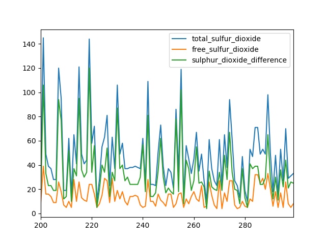
Below a new column called sulphur_dioxide_difference is created that contains the difference between total_sulfur_dioxide and free_sulfur_dioxide
df['sulphur_dioxide_difference'] =
  df['total_sulfur_dioxide'] - df['free_sulfur_dioxide']
print(df.head())
fixed_acidity  volatile_acidity  citric_acid  residual_sugar  chlorides  ...    pH  sulphates  alcohol  quality  sulphur_dioxide_difference
0            7.4              0.70         0.00             1.9      0.076  ...  3.51       0.56      9.4        5                        23.0
1            7.8              0.88         0.00             2.6      0.098  ...  3.20       0.68      9.8        5                        42.0
2            7.8              0.76         0.04             2.3      0.092  ...  3.26       0.65      9.8        5                        39.0
3           11.2              0.28         0.56             1.9      0.075  ...  3.16       0.58      9.8        6                        43.0
4            7.4              0.70         0.00             1.9      0.076  ...  3.51       0.56      9.4        5                        23.0
Plotting
Matplotlib is a comprehensive library for creating static, animated, and interactive visualizations in Python. Pandas has tight integration with matplotlib where data can be displayed from a DataFrame using the plot() method.
df[['total_sulfur_dioxide','free_sulfur_dioxide',
  'sulphur_dioxide_difference']][200:300].plot()
plt.show()

The example above plots 100 samples from the 200 to the 300 element.