Notes about Azure ML, Part 9 - An end-to-end AzureML example Pipeline creation and execution

Sat June 18, 2022

machine-learning azure ml pipeline

Introduction

In the second section of this series, we will show how to use the Azure Machine SDK to create a training pipeline. In the previous section, we uploaded the concrete strength data to an AzureML datastore and published it in a dataset called concrete_baseline. This section will create an AzureML pipeline that will use that dataset to train several models, evaluate their performance, and select the best one.

AzureMl pipelines connect several functional steps we can execute in sequence in a machine learning workflow. They enable development teams to work efficiently as each pipeline step can be developed and optimized individually. The various pipeline steps can be connected using a well-defined interface. Pipelines can be parametrized, thus allowing us to investigate different scenarios and variations of the same AzureML-pipeline.

It is helpful to spend a moment at this stage to discuss the final goal of this Pipeline. We will use this Pipeline to create two models:

a data transformation model that will be used to transform the data into a format that the machine learning model can use.
a machine learning model that will be used to predict the concrete strength of the concrete.

The two models will be used in conjunction in our final deployment. It is also possible to create a single model that will execute both steps, but we opted for the two models approach to show how to use different models together.

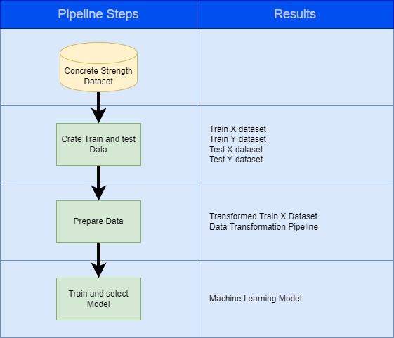
An outline of the Pipeline implemented in this example is shown in the diagram below. The illustration below shows the steps that are part of the Pipeline and the outputs of each step.


Pipeline in this example

The work described in this section is contained in the following folder structure. In the sections below, we will go through all these files individually.

train
│   train_model.py
|   requirements.txt
│
└───src
│   │   data_transformer_builder.py
│   │   model_evaluation.py
|   │   step_prepare_data.py
│   │   step_train_test_split.py
│   │   step_train.py

Data passing mechanisms

There are various options whereby data can be passed from one step to another within an AzureML pipeline; an excellent article on this topic can be found in Vlad Ilescu’s blog [1]. Three options that are available are:

Using AzureMl datasets as pipeline inputs. We have already created a dataset called concrete_baselinethat contains the concrete strength data. We will use this dataset as the input for the first step of the Pipeline.
Using PipelineData. PipelineData is a very versatile object that can be used to pass data of any type between steps in the Pipeline; this is a great choice for passing data that is necessary for the context of the Pipeline. In our example, we will create a dataset with the transformed train features dataset that will also be used as the input to the training step. Similarly, the data preparation model will also be created in the data preparation step and will be used as the input to the training step, albeit it will also be registered as an AzureML model. The natural choice for these entities is the PipelineData object.
Using OutputFileDatasetConfig has many similarities to the PipelineData object, but we can also register it as an AzureML dataset. In our example, we would need to use the train and test datasets in the phases that follow the Pipeline, namely;
- In the model hyperparameter tuning phase, we will use the train datasets as the input to the model hyperparameter tuning step.
- In the validation phase, we will use the test datasets as our input.

Therefore OutputFileDatasetConfig was considered an excellent choice for these cases.

Pipeline steps

In this section, we will look at the steps in more detail. We will also present the code for each step.

Step 1: Creation of Test and Train Datasets

In our experiment, we will base our work on the premise that the amount of cement in our mixture is a vital attribute in predicting the strength of concrete. We will use this information and the stratified sampling technique to create the test and train datasets based on the cement content. This technique will place all records in one of five buckets based on cement content. In practice, we carry out this assignment by creating a temporary field called cement_cat that will hold the cement content bucket. We will then use Scikit Learn’s StratifiedShuffleSplit class to split the data into train and test sets based on cement_cat. The process will yield a test set with a size of 20% and a train set containing 80% of the original data. We will further split the train and test sets into the features and the labels datasets, and the four sets are saved and published as AzureML datasets to be used later on. Naturally, we delete cement_cat at the end of this process.

So, the first pipeline step will use the created concrete_baseline dataset to create the train and test sets and will output four attributes:

train_features: the features dataset for the train set.
train_labels: the labels dataset for the train set.
test_features: the features dataset for the test set.
test_labels: the labels dataset for the test set.

We specify the location of these entities as arguments for this pipeline step, as we shall see later on.

'''
Split Train / Test Pipeline Step
'''
import os
import argparse
import numpy as np
from azureml.core import Run
from sklearn.model_selection import StratifiedShuffleSplit

RANDOM_STATE = 42

run = Run.get_context()

# Parsing the arguments passed to the script.
parser = argparse.ArgumentParser()
parser.add_argument('--train_X_folder', dest='train_X_folder', required=True)
parser.add_argument('--train_y_folder', dest='train_y_folder', required=True)
parser.add_argument('--test_X_folder', dest='test_X_folder', required=True)
parser.add_argument('--test_y_folder', dest='test_y_folder', required=True)
args = parser.parse_args()

Execution of this pipeline step starts with retrieving the concrete_baseline dataset from the AzureML datasets. To do this, we need to get an instance of the current trial’s run context. This is done by calling the get_context() method of the Run class. We can then get the concrete_base dataset through the input_datasets property of the RunContext class, referencing the dataset name. We can convert the dataset to a pandas Dataframe using the to_pandas_dataframe() method so we can use it later on.

# This is the code that is used to read the data from the dataset 
# that was created in the previous step.
concrete_dataset = run.input_datasets['concrete_baseline']
df_concrete = concrete_dataset.to_pandas_dataframe()

As explained above, the concrete_baseline dataset is then split into train and test sets using the StratifiedShuffleSplit class. The StratifiedShuffleSplit class is a cross-validation iterator that provides train/test indices to split data into train/test sets.

# prepare the data, we will use a stratified split to create a train and test set
# first we split the data into 5 buckets according to the cement content
df_concrete['cement_cat'] = np.ceil((df_concrete['cement'] / 540) * 5)

train_set, test_set =  None, None

# we use a stratified split to create a train and test set
split = StratifiedShuffleSplit(n_splits=1, test_size=0.2, random_state=RANDOM_STATE)
for train_idx, test_idx in split.split(df_concrete, df_concrete['cement_cat']):
    train_set = df_concrete.loc[train_idx]
    test_set = df_concrete.loc[test_idx]

# remove cement_cat in train and test datasets
for set_ in (train_set, test_set):
    set_.drop('cement_cat', axis=1, inplace=True)

# This is splitting the data into training and test sets.
X_train = train_set.drop('strength', axis=1)
y_train = train_set['strength'].copy()
X_test = test_set.drop('strength', axis=1)
y_test = test_set['strength'].copy()

The four pandas Dataframes are saved to CSV files in the locations specified as arguments to this pipeline step using the numpy to_csv method. As they were created using the OutputFileDatasetConfig process, they will be automatically registered as AzureML datasets, as we will see later on.

# Write outputs
np.savetxt(os.path.join(args.train_X_folder, "data.txt"), X_test, delimiter=",")
np.savetxt(os.path.join(args.train_y_folder, "data.txt"), y_test, delimiter=",")

np.savetxt(os.path.join(args.test_X_folder, "data.txt"), X_test, delimiter=",")
np.savetxt(os.path.join(args.test_y_folder, "data.txt"), y_test, delimiter=",")

This step also outputs some metrics that the user can use to validate the correct execution using the logging capabilities of the trial’s run. Logging is done through the log() method of the Run class.

# This is logging the shape of the data.

run.log('X_train', X_train.shape)
run.log('y_train', y_train.shape)
run.log('X_test', X_test.shape)
run.log('y_test', y_test.shape)

Step 2: Preparing the Data

In this step, we will use the AzureML SDK and Scikit Learn to prepare the data for training. The result of this step is a Scikit Learn transformation pipeline that will consist of two stages:

A Custom Transformer, called CombinedAggregateAdder, will add coarse and fine aggregate features into a new feature called Aggregate.

'''
Data Transformer Builder

Creates a data transformer comprising of the following steps:

- combines the fine aggregate and coarse aggregate into a single feature
- scales the data using StandardScaler

Transforms the data and returns the transformed data, and the transformer
'''
import numpy as np
from sklearn.base import BaseEstimator, TransformerMixin
from sklearn.pipeline import Pipeline
from sklearn.preprocessing import StandardScaler

coarse_agg_ix, fine_agg_ix = 5, 6

class CombinedAggregateAdder(BaseEstimator, TransformerMixin):
    '''
    sums the aggregate features in the dataset
    '''
    def __init__(self):
        '''
        initializes the class
        '''
        pass

    def fit(self, X, y=None):
        '''
        fit function. returns self
        '''
        return self

    def transform(self, x_val, y_val=None):
        '''
        Transformation function
        '''
        aggregate_total = x_val[:, coarse_agg_ix] + x_val[:, fine_agg_ix]
        x_val = np.delete(x_val, [coarse_agg_ix, fine_agg_ix], axis=1)
        return np.c_[x_val, aggregate_total]

A Standardization Transformer that will standardize the features using Scikit Learn’s StandardScaler.

The two transformers are chained together using Scikit Learn’s Pipeline class. It is essential to mention that this is not the typical approach to preparing the data, as Microsoft Azure provides many tools, such as Azure Databricks, that are better suited for this task. But in our small project, we will use the coding approach.

def transformation_pipeline():
    '''
    Scikit learn Pipeline Creator : the transformer
    '''
    # Creating a pipeline that will first add the
    # two aggregate features and then scale the data.
    pipeline = Pipeline([
        ('CombinedAggregateAdder', CombinedAggregateAdder()),
        ('StandardScaler', StandardScaler())
    ])

    return pipeline

The code to generate the data transformation pipeline is shown below. The method pipeline_fit_transform_save() is used return the the pipeline and transformed data.


def data_transform(data):
    '''
    Creates a transformation pipeline using data.
    Returns the transformed data and the Pipeline.
    '''
    data_transformer = transformation_pipeline()
    transformed_data = data_transformer.fit_transform(data)

    return data_transformer, transformed_data

The second step of the Pipeline will use the transformation specified above to prepare the data for training. As mentioned previously, this step will create a Scikit learn data preparation pipeline that we will use to transform our data so that our machine learning model can use it. This data preparation pipeline will be registered as an AzureML model that can be easily loaded and used in other phases of this project in conjunction with the Machine Learning Model.

This pipeline step has three arguments.

An input argument, the training features dataset location.
Two output arguments; the transformed training features dataset location and the data preparation pipeline location.

In this approach, we will be passing the location of the data preparation pipeline and the transformed features data as pipeline parameters. Nonetheless, as we have seen previously, other methods are possible.

'''
Data Preprocessor step of the Pipeline.
'''
import os
import argparse
import pickle
import numpy as np
import pandas as pd
from azureml.core import Run
from data_transformer_builder import data_transform

# The dataset is specified at the pipeline definition level.
run = Run.get_context()

# Parsing the arguments passed to the script.
parser = argparse.ArgumentParser()
parser.add_argument('--train_X_folder', dest='train_X_folder', required=True)
parser.add_argument('--train_Xt_folder', dest='train_Xt_folder', required=True)
parser.add_argument('--data_transformer_folder', dest='data_transformer_folder', required=True)
args = parser.parse_args()

# Loading the data from the data store.
X_train_path = os.path.join(args.train_X_folder, "data.txt")
X_train = pd.read_csv(X_train_path, header=None).to_numpy()
run.log('X_train', X_train.shape)

The pipeline step will call the pipeline_fit_transform_save(), passing the train features data to obtain the data-transformer and the transformed data features. The transformed data is then saved to the specified location and registered as an AzureML model.

# Fitting the data transformer to the training data.
data_transformer, X_train_transformed = data_transform(X_train)
run.log('X_train_transf', X_train_transformed.shape)
run.log('data_transformer', data_transformer)

Finally, we save the data-transformer to the specified location and register it as an AzureML model with the name data_transformer. We also save the transformed data to its specified location so that it can be used in the next step of the Pipeline.

if not os.path.exists(args.train_Xt_folder):
    os.mkdir(args.train_Xt_folder)

# Saving the transformed data to the data store.
np.savetxt(
    os.path.join(args.train_Xt_folder, "data.txt"),
    X_train_transformed,
    delimiter=",",
    fmt='%s')

if not os.path.exists(args.data_transformer_folder):
    os.mkdir(args.data_transformer_folder)

# Saving the transformer to a file.
data_transformer_path = os.path.join(args.data_transformer_folder, 'data_transformer.pkl')
with open(data_transformer_path, 'wb') as handle:
    pickle.dump(data_transformer, handle, protocol=pickle.HIGHEST_PROTOCOL)

# Registering the model in the Azure ML workspace.
run.upload_file(data_transformer_path,data_transformer_path)
run.register_model(model_path=data_transformer_path, model_name='data_transformer')

Step 3: Train and select the Model

The last step of the Pipeline is to train several models, evaluate their performance and select the best one. The models that are considered are the following:

Linear Regression, using Scikit Learn’s LinearRegression class.
Random Forest, using Scikit Learn’s RandomForestRegressor class.
Gradient Boosting, using Scikit Learn’s GradientBoostingRegressor class.
Bagging Regressor, using Scikit Learn’s BaggingRegressor class.

The models are evaluated using the root mean squared error (RMSE) metric, where

$$RMSE = \sqrt{\frac{1}{n}\sum_{i=1}^{n}(y_i - \hat{y_i})^2}$$

, where $y_i$ is the actual value and $\hat{y_i}$ is the predicted value for the ith test record.

Let us break down the code of this step.

We start the development of this step by creating the cost function to be used for the model evaluation. The code presented is very straightforward; the predicted values are calculated from the model and compared to the test-lables. Obviously, this is not the only or best way to evaluate our models.

'''
Evaluation functions for the model
'''
import numpy as np
from sklearn.metrics import mean_squared_error

def rmse_evaluate(model, X_val, y_val):
    '''
    Calculates the root of the mean squared error of the model
    '''
    # Calculating the root of mean squared error of the model.
    prediction = model.predict(X_val)
    test_mse = mean_squared_error(y_val, prediction)
    sqrt_mse = np.sqrt(test_mse)
    return sqrt_mse

Next, we present the training step code. The code is very similar in nature to what we presented in the previous steps; however there are some differences:

This Pipeline step will use some pipeline arguments that will allow us to modify some of the models' hyperparameters at this stage, thus helping us in selecting the best model. This step has the following arguments:
- train_y_folder, the location of the training labels that we have previously stored in a data store.
- train_Xt_folder, the location of the transformed training features that we have previously stored in a data store.
- model_folder, the location where the model that we will select in this step will be saved.
- bag_regressor_n_estimators, the number of trees in the bagging regressor. This is a pipeline argument that will have an initial value that we will define during pipeline creation. This argument, as we shall see later on, can be modified so that a new selection trial is carried out without resubmitting the entire pipeline code.
- decision_tree_max_depth, the maximum depth of the decision tree. Similar to the argument above, this is a pipeline argument.
- random_forest_n_estimators, the number of trees in the random forest. Similar to the argument above, this is a pipeline argument.

'''
Train step. Trains various models and selects the best one.
'''
import os
import argparse
import pickle
import pandas as pd
from azureml.core import Run
from sklearn.ensemble import BaggingRegressor, RandomForestRegressor
from sklearn.linear_model import LinearRegression
from sklearn.tree import DecisionTreeRegressor
from model_evaluation import evaluate

# Getting the run context.
run = Run.get_context()

# Parsing the arguments passed to the script.
parser = argparse.ArgumentParser()
parser.add_argument('--train_y_folder', dest='train_y_folder', required=True)
parser.add_argument('--train_Xt_folder', dest='train_Xt_folder', required=True)
parser.add_argument('--model_folder', dest='model_folder', required=True)

parser.add_argument(
    '--bag_regressor_n_estimators',
    dest='bag_regressor_n_estimators',
    required=True)
parser.add_argument(
    '--decision_tree_max_depth',
    dest='decision_tree_max_depth',
    required=True)
parser.add_argument(
    '--random_forest_n_estimators',
    dest='random_forest_n_estimators',
    required=True)
args = parser.parse_args()

# Reading the data from the `X_train_trans.txt` file and converting it to a numpy array.
X_t_path = os.path.join(args.train_Xt_folder, "data.txt")
X_train_trans = pd.read_csv(X_t_path, header=None).to_numpy()

# Reading the data from the `y_train.txt` file and converting it to a numpy array.
y_path = os.path.join(args.train_y_folder, "data.txt")
y_train = pd.read_csv(y_path, header=None).to_numpy()

This step loads the training labels and the transformed training features from the data store and executes the training of the models. The models are assigned the hyperparameters that we have specified during the pipeline creation. Obviously, we could have added more parameters to have better criteria for selecting our model, but we have chosen to keep the number of parameters as low as possible.
The cost function is evaluated for each model and logged to the pipeline step metrics by using the run.log() function. We also store the model and the resulting RMSE in a dictionary.

# Creating an empty dictionary.
results = {}

# Training a linear regression model and evaluating it.
lin_regression = LinearRegression()
lin_regression.fit(X_train_trans, y_train)
sqrt_mse= evaluate(lin_regression, X_train_trans, y_train)
results[lin_regression] = sqrt_mse
run.log('LinearRegression', sqrt_mse)

# Training a bagging regressor model and evaluating it.
bag_regressor = BaggingRegressor(
    n_estimators=int(args.bag_regressor_n_estimators),
    random_state=42)
bag_regressor.fit(X_train_trans, y_train)
sqrt_mse= evaluate(bag_regressor, X_train_trans, y_train)
results[bag_regressor] = sqrt_mse
run.log('BaggingRegressor', sqrt_mse)

# Training a decision tree regressor model and evaluating it.
dec_tree_regressor = DecisionTreeRegressor(
    max_depth=int(args.decision_tree_max_depth))
dec_tree_regressor.fit(X_train_trans, y_train)
sqrt_mse= evaluate(dec_tree_regressor, X_train_trans, y_train)
results[dec_tree_regressor] = sqrt_mse
run.log('DecisionTreeRegressor',sqrt_mse)

# Training a random forest regressor model and evaluating it.
random_forest_regressor = RandomForestRegressor(
    n_estimators=int(args.random_forest_n_estimators),
    random_state=42)
random_forest_regressor.fit(X_train_trans, y_train)
sqrt_mse= evaluate(random_forest_regressor, X_train_trans, y_train)
results[random_forest_regressor] = sqrt_mse
run.log('RandomForestRegressor', sqrt_mse)

The selected model is obtained by looking for the minimum RMSE in the dictionary. The selected model name is also logged to the pipeline step metrics.

# Selecting the model with the lowest RMSE.
selected_model =  min(results, key=results.get)
run.log('selected_model', selected_model)

Finally, the selected model is saved to the data store in the location specified by the model_folder argument. The model is also registered in the AzureML workspace with the name of concrete_model.


if not os.path.exists(args.model_folder):
    os.mkdir(args.model_folder)

# Saving the model to a file.
model_path = os.path.join(args.model_folder, 'model.pkl')
with open(model_path, 'wb') as handle:
    pickle.dump(selected_model, handle, protocol=pickle.HIGHEST_PROTOCOL)

# Uploading the model to the Azure ML workspace and registering it.
run.upload_file(model_path,model_path)
run.register_model(model_path=model_path, model_name='concrete_model')

Putting it all together - Pipeline creation

Finally, all this work comes together when we create the Pipeline that will be used to train the model. We start this process by

getting an instance of our AzureML workspace. In order to do this, we will use the configuration file that we created when we created the workspace.
creating a RunConfiguration object. This object will be used to specify the configuration of the Pipeline.
defining an Environment object. This object will be used to specify the environment in which the Pipeline will be executed. In our case, we will create the environment from a pip specification file. This specification file contains the list of packages that will be used in the Pipeline and is as follows:

scikit-learn
pandas
azureml-core
azureml-dataset-runtime
azureml-defaults

we then assign the environment attribute of our RunConfiguration object to the created Environment object.

'''
Execute the training pipeline with the following steps:

- Step 1: Split the data into train and test sets
- Step 2: Prepare the train data for training and generate a prepare-data pipeline
- Step 3: Train the model using various algorithms and select the best one
'''
import os
from azureml.pipeline.steps.python_script_step import PythonScriptStep
from azureml.pipeline.core import Pipeline, PipelineParameter
from azureml.core import Workspace, Experiment, Dataset, Datastore
from azureml.core.runconfig import RunConfiguration
from azureml.core.environment import Environment
from azureml.pipeline.core import PipelineData
from azureml.data.output_dataset_config import OutputFileDatasetConfig
from azuremlproject import constants

# Loading the workspace from the config file.
config_path = os.path.join(
    os.path.dirname(os.path.realpath(__file__)),
    '..',
    '..',
    '.azureml')
ws = Workspace.from_config(path=config_path)

# create a new run_config object
run_config = RunConfiguration()

# Creating a new environment with the name concrete_env and 
# installing the packages in the requirements.txt file.
environment = Environment.from_pip_requirements(
    name='concrete_env',
    file_path=os.path.join(
        os.path.dirname(os.path.realpath(__file__)),
        'requirements.txt')
    )
run_config.environment = environment

We then specify the location of source files containing the pipeline steps. This folder is uploaded to the AzureML workspace so that the Pipeline is created and executed. This location is during the creation of each pipeline step.

# Path to the folder containing the scripts that
# will be executed by the pipeline.
source_directory = os.path.join(
    os.path.dirname(os.path.realpath(__file__)),
    'src')

We also get a reference to the AzureML data store that will be used to store the various assets that will be created by this Pipeline. As discussed earlier, we will use the data store that we created during the creation of the workspace, whose name is specified in a constants file.

data_store = Datastore(ws, constants.DATASTORE_NAME)

We then define the entities that will hold our assets as described previously.

We will use the OutputFileDatasetConfig class to store the train and test features and labels. We also use the register_on_complete method to register the train and test features and labels as AzureML datasets.
We use the PipelineData class to store the transformed train features as this data is not required outside the Pipeline.
We use the PipelineData class to store the data_transformer and the selected model. These items will be registered as AzureML models when they are created.

train_X_folder = OutputFileDatasetConfig(
    destination=(data_store, 'train_X_folder')).register_on_complete('train_X')
train_y_folder = OutputFileDatasetConfig(
    destination=(data_store, 'train_y_folder')).register_on_complete('train_y')

test_X_folder = OutputFileDatasetConfig(
    destination=(data_store, 'test_X_folder')).register_on_complete('test_X')

test_y_folder = OutputFileDatasetConfig(
    destination=(data_store, 'test_y_folder')).register_on_complete('test_y')

train_Xt_folder = PipelineData('train_Xt_folder', datastore=data_store, is_directory=True)

data_transformer_folder = PipelineData('data_transformer_folder', datastore=data_store)
model_folder = PipelineData('model_folder', datastore=data_store)

Next, we get an instance of the concrete_baseline dataset that we created earlier. This data is the starting point of our Pipeline and will be used to drive the entire process.

concrete_dataset = Dataset.get_by_name(ws, 'concrete_baseline')
ds_input = concrete_dataset.as_named_input('concrete_baseline')

Next, we create the pipeline steps using the PythonScriptStep class. The constructor of this class takes the following arguments:

Name of the script file that contains the code for this step.
A list of arguments that will be passed to the script.
A list of input arguments that will be used by the script.
A list of output arguments that will be generated by the script.
The compute where the script will be executed. As explained earlier, instance and target computes are created during the creation of the workspace and have their names specified in a constants file. The pipeline steps are executed in the compute instance.
The instance of the run configuration that will be used to configure the execution of the Pipeline.


step_train_test_split = PythonScriptStep(
    script_name='step_train_test_split.py',
    arguments=[
        '--train_X_folder', train_X_folder,
        '--train_y_folder', train_y_folder,
        '--test_X_folder', test_X_folder,
        '--test_y_folder', test_y_folder],
    inputs=[
        ds_input],
    outputs=[
        train_X_folder,
        train_y_folder,
        test_X_folder,
        test_y_folder],
    compute_target=constants.INSTANCE_NAME,
    source_directory=source_directory,
    runconfig=run_config
)

step_prepare_data = PythonScriptStep(
    script_name='step_prepare_data.py',
    arguments=[
        '--train_X_folder', train_X_folder,
        '--train_Xt_folder', train_Xt_folder,
        '--data_transformer_folder', data_transformer_folder],
    outputs=[
        train_Xt_folder,
        data_transformer_folder],
    inputs=[train_X_folder],
    compute_target=constants.INSTANCE_NAME,
    source_directory=source_directory,
    runconfig=run_config
)

The final step of our pipeline uses several pipeline parameters that give us the flexibility to fine-tune the various models so that we can select the best one. We use the PipelineParameter class to create these parameters, giving them names and default values.


param_bag_regressor_n_estimators = PipelineParameter(
    name='The number of estimators of the bagging regressor',
    default_value=20)

param_decision_tree_max_depth = PipelineParameter(
    name='The maximum depth of the decision tree',
    default_value=5)

param_random_forest_n_estimators = PipelineParameter(
    name='The number of estimators of the random forest',
    default_value=5)

training_step = PythonScriptStep(
    script_name='step_train.py',
    arguments=[
        '--train_Xt_folder', train_Xt_folder,
        '--train_y_folder', train_y_folder,
        '--model_folder', model_folder,
        '--bag_regressor_n_estimators', param_bag_regressor_n_estimators,
        '--decision_tree_max_depth', param_decision_tree_max_depth,
        '--random_forest_n_estimators', param_random_forest_n_estimators],
    inputs=[
        train_Xt_folder,
        train_y_folder],
    outputs=[
        model_folder],
    compute_target=constants.INSTANCE_NAME,
    source_directory=source_directory,
    runconfig=run_config
)

We can now create a pipeline that will execute the steps in the order that we defined them by using the Pipeline class. The constructor of this class takes the following arguments:

the workspace where the Pipeline will be created.
a list of steps that will be executed in the order that they are defined.

We can then execute the Pipeline by creating an Experiment object and calling the submit() method.

pipeline = Pipeline(
    workspace=ws,
    steps=[
        step_train_test_split,
        step_prepare_data,
        training_step
    ])

experiment = Experiment(ws, 'concrete_train')
run = experiment.submit(pipeline)
run.wait_for_completion()

Execution

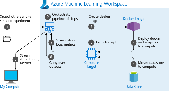
When a pipeline is first executed, AzureML does a couple of things [3]:

Downloads the project to the compute from the Blob storage associated with the workspace.
Builds a Docker image corresponding to each step in the Pipeline.
Downloads the Docker image for each step to the compute from the container registry.
Configures access to Dataset and OutputFileDatasetConfig objects.
Runs the step in the compute target specified in the step definition.
Creates artefacts, such as logs, stdout and stderr, metrics, and output specified by the step. These artefacts are then uploaded and kept in the user’s default datastore.


Running experiment as a pipeline process - Image from Microsoft

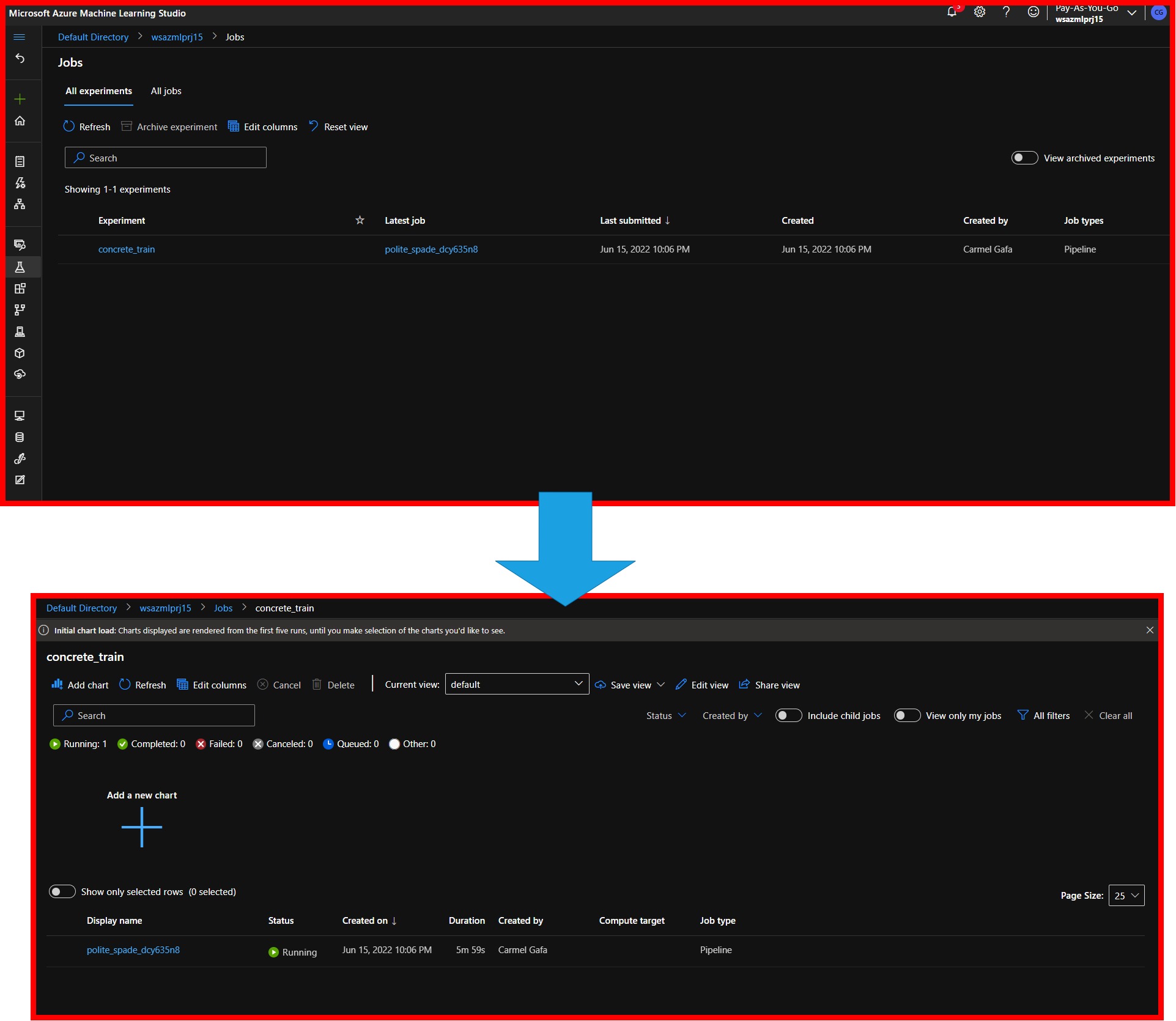
Navigating into the AzureML portal, we will be able to see the experiment name (concrete_train) in the experiments tab, and upon clicking on it, we will see the various trials that were executed.


Experiment in AzureML

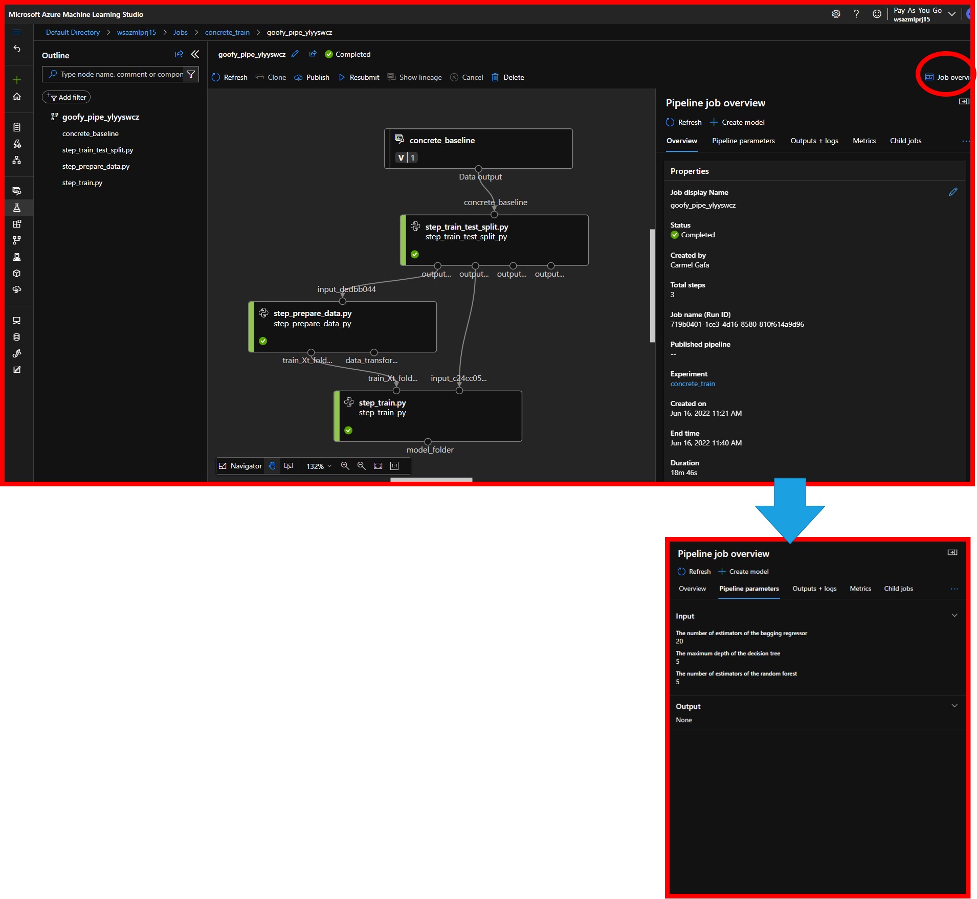
Each trial will show a pictorial representation of the execution steps of the Pipeline, with an indication of whether the step was executed correctly (green marker) or if an error was encountered(red marker). We can also view some general information about the Pipeline, the pipeline parameters that were used for the trial, log files for the execution, the pipeline metrics and information about any jobs that were triggered by the Pipeline.


AzureML pipeline visualization

Navigation to each pipeline step, we can obtain more information about the execution of the step. Each step has a number of tabs, including:

An overview will give us generic information such as the execution time for the step, the name of the script for the step, and the arguments used.
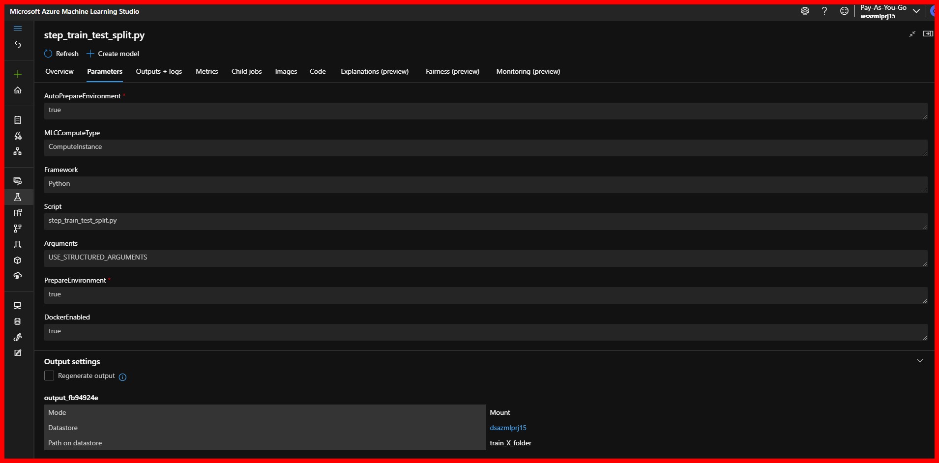
Parameters information, including the location of each argument.
Complete Logging for the execution of the step.
Metrics, or the information that we had logged using the run.log() method in the pipeline


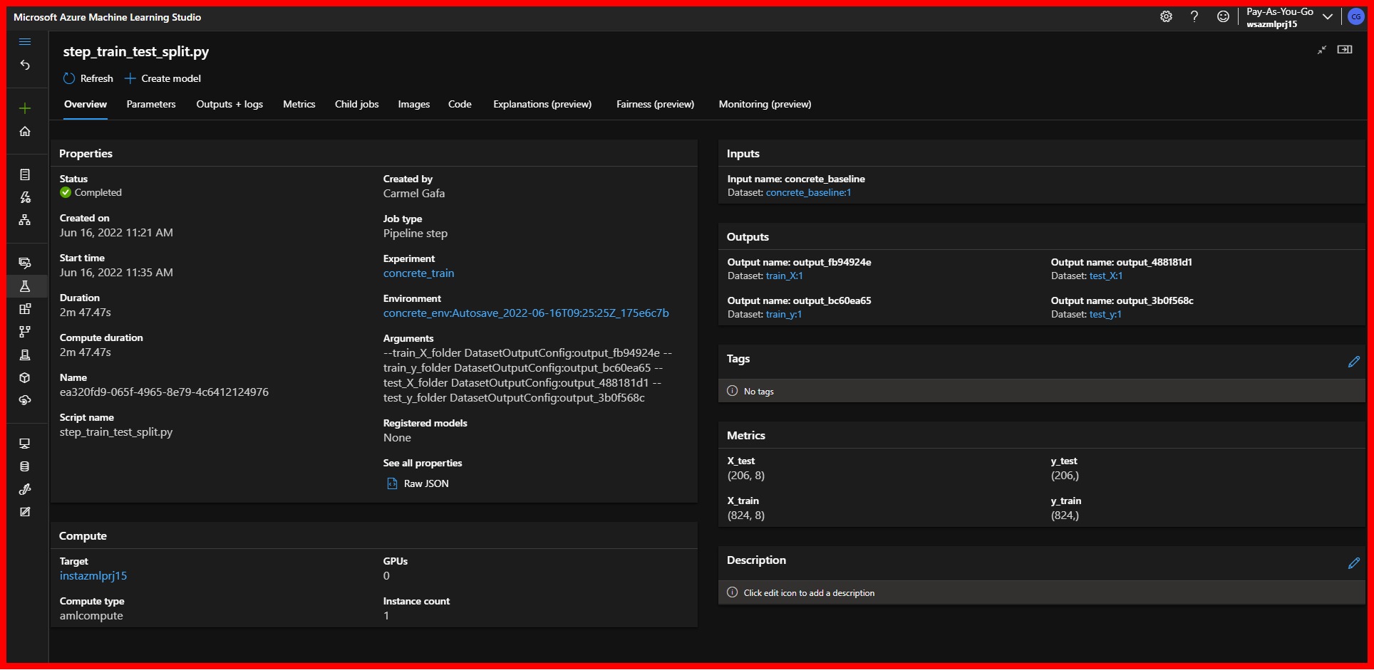AzureML Pipeline Step Overview


AzureML Pipeline Step Overview


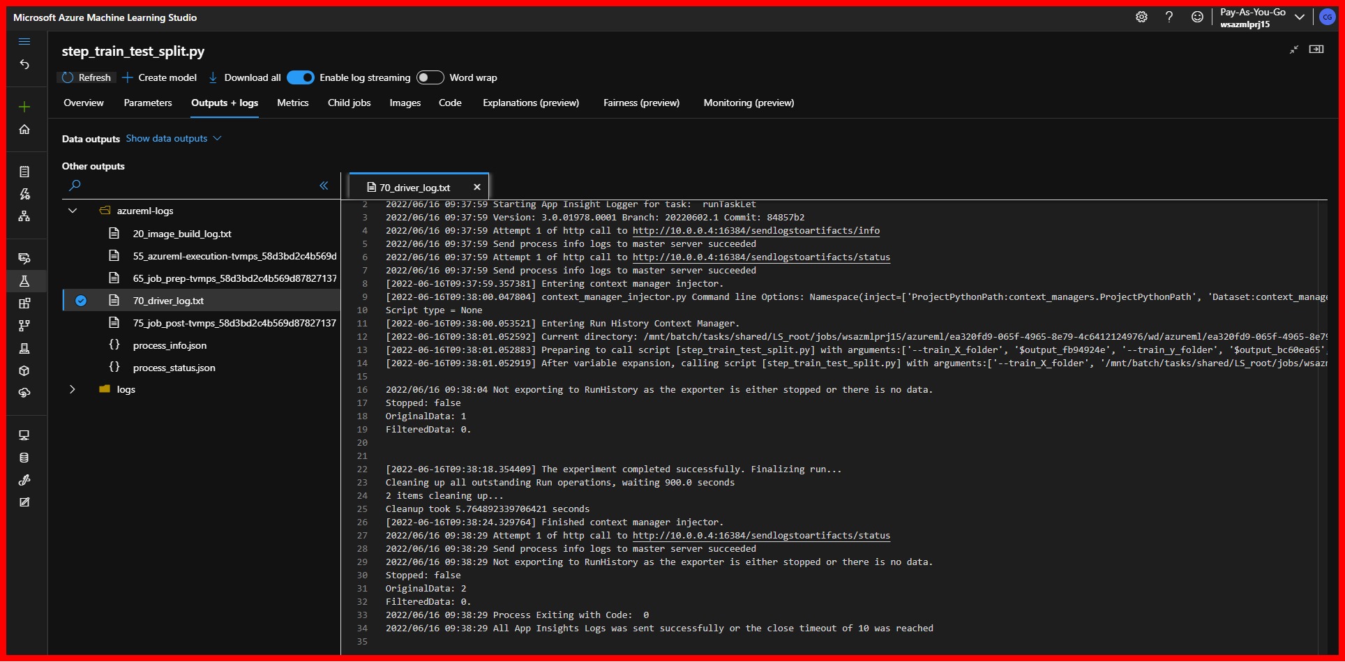AzureML Pipeline Step Logs


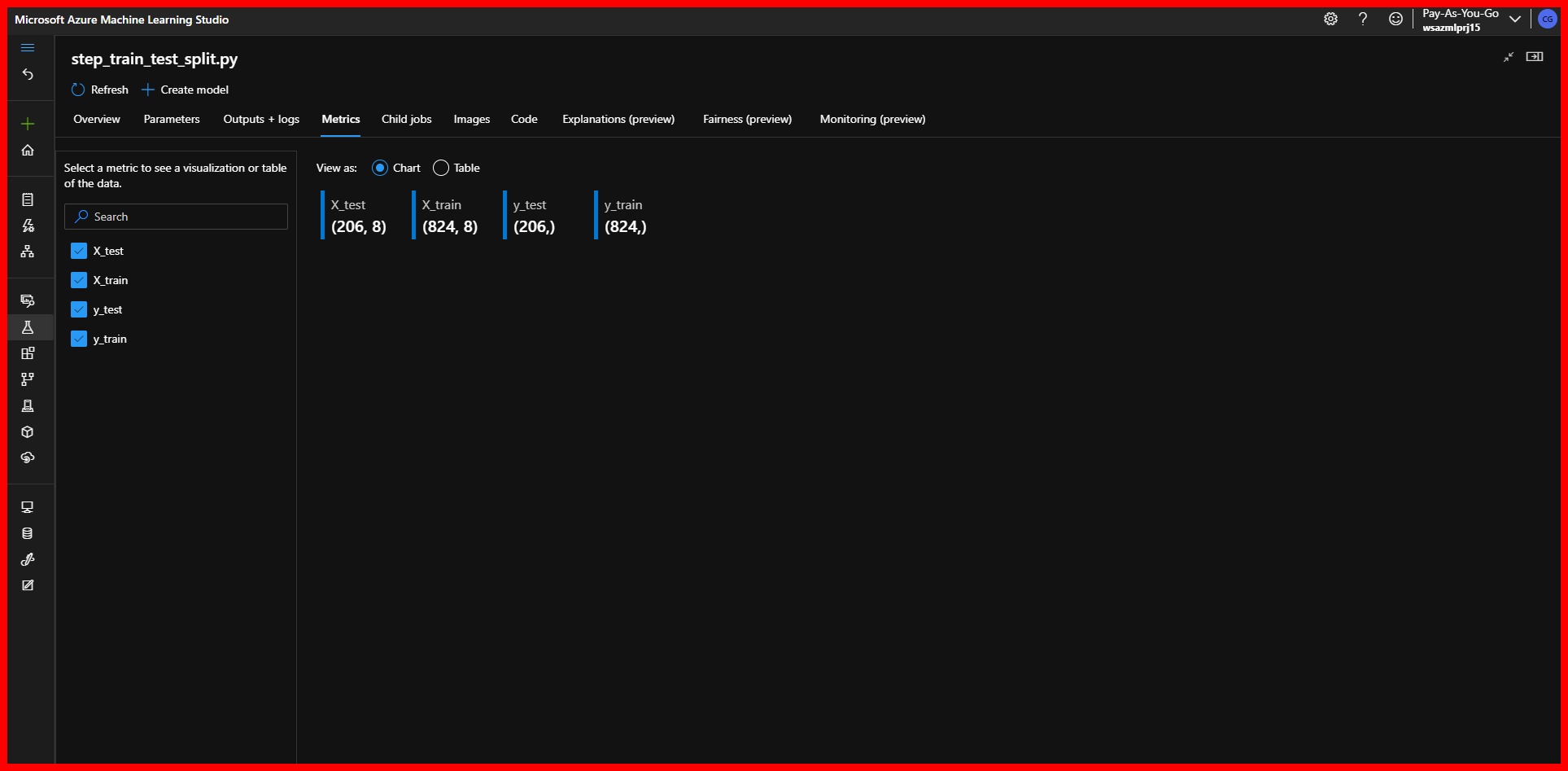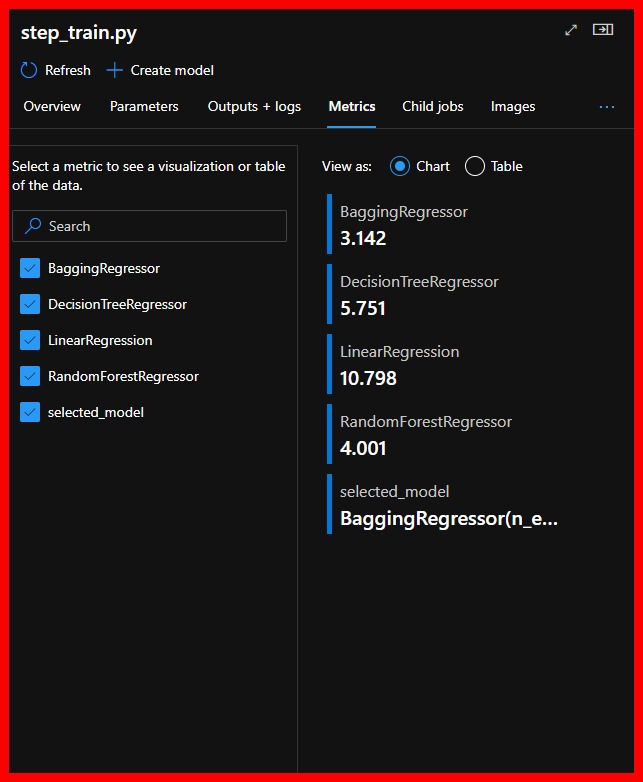
AzureML Pipeline Step Metrics

The metrics of the final step will show us the result of this Pipeline. We can see that the Bagging Regressor obtained the lowest Root Mean Square Error and therefore was saved as our selected model.


Results for this Pipeline

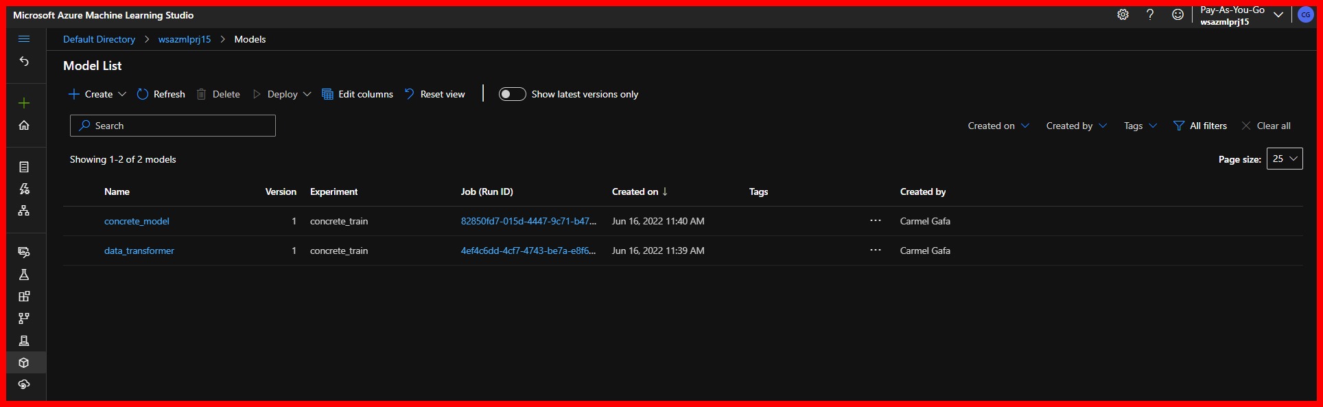
We can have a look at the models that were registered in the workspace during the execution of the Pipeline by navigating to the Models tab. We can verify that two models were registered, one for the data transformer and one for the Bagging regressor model.


Models registered by Pipeline

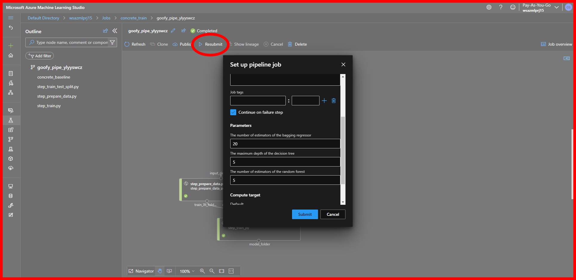
Finally, it is possible to re-run the Pipeline with different parameters without resubmitting the code by selecting the Resubmit option for the Pipeline. This will give us the option to input new values for the parameters and re-run the Pipeline in a new trial.


Pipeline Resubmit

Conclusion

In this post, we have seen how we can create and execute a pipeline in AzureML that tests various ML models and selects the best one. We have seen that for our dataset, with the transformations that we applied, the Bagging Regressor obtained the lowest Root Mean Square Error of 3.142.

In the next post, we will see how AzureMl can optime the model so that we can deploy the best possible model to our production environment.

References

[1] V. Iliescu, Vlad Iliescu [Online]. [Accessed: June 08, 2022].
[2] Li et al, Use pipeline parameters to build versatile pipelines - azure machine learning | Microsoft Docs. [Online]. [Accessed: June 09, 2022].
[3] Nils Pohlmann. (n.d.).Create and run ML pipelines - azure machine learning. Create and run ML pipelines - Azure Machine Learning | Microsoft Docs. [Online]. [Accessed June 17, 2022]