We started this series of posts with an examination of Cost Functions, and then moved on to derive and implement the solution to the linear regression problem for a single variable We extended this to a multi-variable linear regression problem, and we derived and implemented the solution for this case. Our final comment was that as the number of variables increases, the solution becomes computationally prohibitive.
In this post, we will look at gradient descent, an iterative optimization algorithm used to find the minimum of a function. The basic idea is to iteratively move in the opposite direction of the gradient at a given point, thus moving in the direction of the steepest descent.
Recap of the univariate linear regression problem
We have seen in the previous posts that given a hypothesis function.
$$ a_0 + a_1 x $$
we can vary our parameters $a_0$ and $a_1$ minimize a cost function. The cost function that we used in the previous posts is the Mean Square Error,
$$MSE = \frac{\sum_{i=1}^{n} ( \hat{y}_i-y_i )^{2} }{n}$$
In this post, we will use a slightly different version of MSE, that is,
$$MSE = \frac{\sum_{i=1}^{n} ( \hat{y}_i-y_i )^{2} }{2n}$$
The purpose of the factor of two in the denominator is to simplify the calculations that we will meet further on. Adding a factor of two to the denominator does not modify the effect of the cost function, but as the MSE contains a squared term, the derivation will produce a factor of two in the numerator. Having a scaled MSE will mean that the factor of 2 will cancel out when deriving.
Gradient Descent
The basic algorithm for gradient descent is simple, and we will use the following notation:
- start initial values for the parameters $a_0$ and $a_1$
- keep changing the parameters until the cost function is minimized
We can formally write the algorithm as follows:
repeat until convergence
- $$ a_0 := a_0 - \alpha \frac{\partial}{\partial a_0} MSE(a_0, a_1)$$
- $$ a_1 := a_1 - \alpha \frac{\partial}{\partial a_1} MSE(a_0, a_1)$$
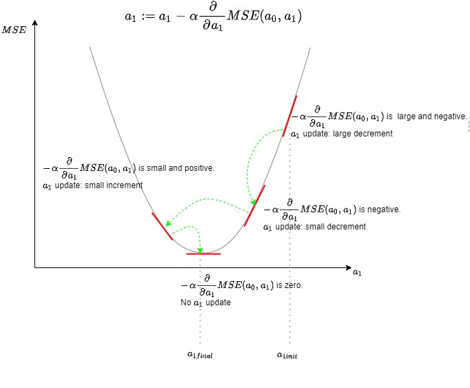
We will update the two parameters simultaneously, and the cost function is evaluated at each iteration. A visual representation of the algorithm for one parameter, in this case, $a_1$ is shown below.
A note about the value of $\alpha$
The value of $\alpha$ is the step size. It affects the precision and the speed of convergence and should be tuned to the problem at hand.
- The smaller the step size, the more accurate the solution will be, but the longer it will take to converge. The more significant the step size, the gradient descent can overshoot and may fail to converge or diverge.
One important thing to note is that the term,
$$ \alpha \frac{\partial}{\partial a} MSE(a_0, a_1)$$
will become smaller in magnitude as a result moves closer to a minimum. Hence, gradient descent will take smaller stems as a local minimum is approached, and therefore there is no need to adjust the step size by adjusting $\alpha$.
Gradient Descent for Linear Regression
We have seen that the function that we want to minimize is
$$MSE(a_0, a_1) = \frac{\sum_{i=1}^{n} ( \hat{y}_i-y_i )^{2} }{2n}$$
Differentiating this function with respect to $a_0$ gives us:
$$\frac{\partial MSE(a_0, a_1)}{\partial a_0} = \frac{\partial}{\partial a_0} \frac{\sum_{i=1}^{n} ( \hat{y}_i-y_i )^2}{2n}$$
$$ = \frac{\partial}{\partial a_0} \frac{\sum_{i=1}^{n} (a_0 + a_1 x_i - y_i)^2}{2n}$$
$$ = \frac{\sum_{i=1}^{n} 2(a_0 + a_1 x_i - y_i)(1)}{2n}$$
$$ = \frac{\sum_{i=1}^{n} (a_0 + a_1 x_i - y_i)}{n}$$
$$ = \frac{\sum_{i=1}^{n} ( \hat{y}_i-y_i)}{n}$$
and similarly for $a_1$.
$$\frac{\partial MSE(a_0, a_1)}{\partial a_0} = \frac{\partial}{\partial a_1} \frac{\sum_{i=1}^{n} ( \hat{y}_i-y_i )^2}{2n}$$
$$ = \frac{\partial}{\partial a_1} \frac{\sum_{i=1}^{n} (a_0 + a_1 x_i - y_i)^2}{2n}$$
$$ = \frac{\sum_{i=1}^{n} 2(a_0 + a_1 x_i - y_i)(x_i)}{2n}$$
$$ = \frac{\sum_{i=1}^{n} (x_i)(a_0 + a_1 x_i - y_i)}{n}$$
$$ = \frac{\sum_{i=1}^{n} (x_i)(\hat{y}_i-y_i)}{n}$$
Therefore, our algorithm becomes the following:
repeat until convergence
- $$ a_0 := a_0 - \frac{\alpha}{n} \sum_{i=1}^{n} ( \hat{y}_i-y_i)$$
- $$ a_1 := a_1 - \frac{\alpha}{n} \sum_{i=1}^{n} ( \hat{y}_i-y_i)(x_i)$$
Gradient Descent for Univariate Linear Regression - Python Implementation
In a previous post, we implemented the linear regression algorithm for the single variable problem. Below is an implementation the gradient descent algorithm for a univariate linear regression problem using Python.
import os
import numpy
import matplotlib
matplotlib.rcParams['text.usetex'] = True
import matplotlib.pyplot as plt
class UnivariateGradientDescent:
'''
Gradient Descent Univariate utilizing numpy
not very efficient but easier to follow
'''
def __init__(self, alpha):
self.__a0 = -5
self.__a1 = -3
self.__training_data = []
self.__alpha = alpha
self.__threshold_iterations = 100000
self.__threshold_cost = 12
def __load_training_data(self, file):
'''
Loads the training data from a file
'''
current_directory = os.path.dirname(__file__)
full_filename = os.path.join(current_directory, file)
self.__training_data = numpy.loadtxt(full_filename, delimiter=',', skiprows=1)
def get_y_value(self, x_value):
'''
return an estimated y value given an x value based on the training results
'''
return self.__calculate_hypothesis(x_value)
def train(self, file):
'''
starts the training procedure
'''
self.__load_training_data(file)
counter = 1
cost = 0
costs = []
a_1s = []
while True:
cost = self.__calculate_cost_function()
counter += 1
costs.append(cost)
a_1s.append(self.__a1)
if cost < self.__threshold_cost or counter > self.__threshold_iterations:
print(f'Cost Function: {cost}')
print(f'Iterations: {counter}')
break
plt.rcParams['text.usetex'] = True
plt.plot(a_1s[:], costs[:], '--bx', color='lightblue', mec='red')
plt.xlabel('a1')
plt.ylabel('cost')
plt.title(r'Cost Function vs. a1, with $\alpha$ =' + str(self.__alpha))
plt.show()
def __calculate_cost_function(self):
'''
returns the cost function
'''
training_count = len(self.__training_data)
sum_a0 = 0.0
sum_a1 = 0.0
sum_cost = 0.0
cost = 0.0
for idx in range(0, training_count):
y_value = self.__training_data[idx][1]
x_value = self.__training_data[idx][0]
y_hat = self.__calculate_hypothesis(x_value)
sum_a0 += (y_hat - y_value)
sum_a1 += ((y_hat - y_value) * x_value)
sum_cost += pow((y_hat - y_value), 2)
self.__a0 -= ((self.__alpha * sum_a0) / training_count)
self.__a1 -= ((self.__alpha * sum_a1) / training_count)
cost = ((1 / (2 * training_count)) * sum_cost)
return cost
def __calculate_hypothesis(self, x_value):
'''
calculates the hypothesis for a value of x
'''
hypothesis = self.__a0 + (self.__a1 * x_value)
return hypothesis
def print_hypothesis(self):
'''
prints the hypothesis equation
'''
print(f'y = {self.__a0} x + {self.__a1}')
if __name__ == '__main__':
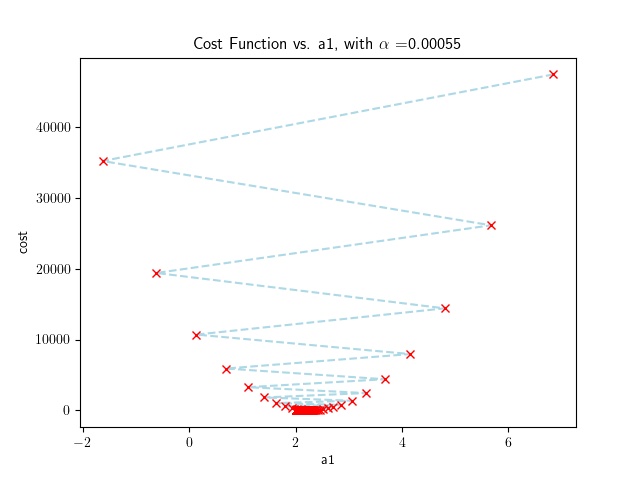
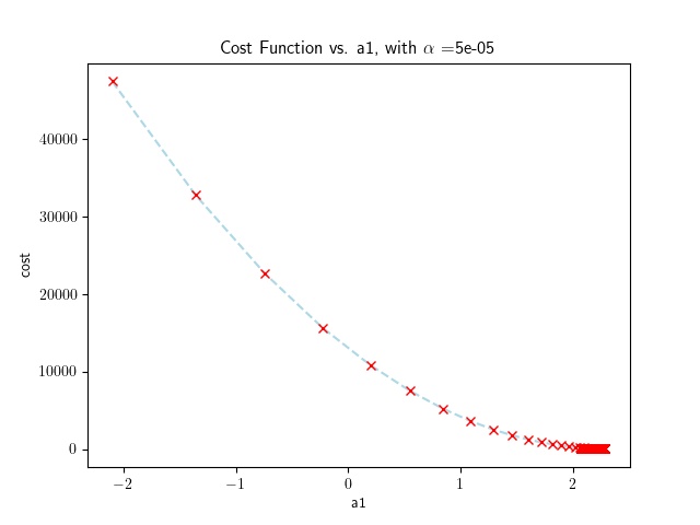
gradient_descent = UnivariateGradientDescent(0.00005)
gradient_descent.train('data.csv')
gradient_descent.print_hypothesis()
The program plots the values of $a_1$ with the cost function as the algorithm converges. It is then possible to see the effect of the learning rate on the convergence. For example a reasonably large learning rate will produce the following results:
Whereas a small learning rate will produce the following results:
A variation of the program, using pandas, is shown below. In this case the program is comparing the decrease of the cost function and using the difference as a stopping criteria.
import os
import matplotlib
matplotlib.rcParams['text.usetex'] = True
import matplotlib.pyplot as plt
import pandas as pd
import sys

class UnivariateGradientDescent:
    '''
    Gradient Descent Univariate utilizing pandas
    '''

    def __init__(self, alpha):
        self.__a0 = 5
        self.__a1 = 3
        self.__training_data = []

        self.__alpha = alpha
        self.__threshold_iterations = 100000


    def __load_training_data(self, file):
        full_filename = os.path.join(os.path.dirname(__file__), file)
        self.__training_data = pd.read_csv(full_filename, delimiter=',', names=['x', 'y'], index_col=False)

    def get_y_value(self, x_value):
        '''
        return an estimated y value given an x value based on the training results
        '''
        return self.__calculate_hypothesis(x_value)

    def train(self, file):
        '''
        starts the training procedure
        '''
        self.__load_training_data(file)
        m = len(self.__training_data)
        iterations = 0

        previous_cost = sys.float_info.max

        costs = []
        a_1s = []

        while True:
            # calculate the hypothesis function for all training data
            self.__training_data['y_hat'] = self.__a0 + (self.__a1 * self.__training_data['x'])

            # calculate the difference between the hypothesis function and the
            # actual y value for all training data
            self.__training_data['y_hat-y'] = self.__training_data['y_hat'] - self.__training_data['y']

            # multiply the difference by the x value for all training data
            self.__training_data['y-hat-y.x'] = self.__training_data['y_hat-y'] * self.__training_data['x']

            # square the difference for all training data
            self.__training_data['y-hat-y_sq'] = self.__training_data['y_hat-y'] ** 2

            # update the a0 and a1 values
            self.__a0 -= (self.__alpha * (1/m) * sum(self.__training_data['y_hat-y']))
            self.__a1 -= (self.__alpha * (1/m) * sum(self.__training_data['y-hat-y.x']))

            # calculate the cost function
            cost = sum(self.__training_data['y-hat-y_sq']) / (2 * m)
            iterations += 1

            # record the cost and a1 values for plotting
            costs.append(cost)
            a_1s.append(self.__a1)

            cost_difference = previous_cost - cost
            print(f'Iteration: {iterations}, cost: {cost:.3f}, difference: {cost_difference:.6f}')
            previous_cost = cost

            # check if the cost function is diverging, if so, break
            if cost_difference < 0:
                print(f'Cost function is diverging. Stopping training.')
                break

            # check if the cost function is close enough to 0, if so, break or if the number of
            # iterations is greater than the threshold, break
            if abs(cost_difference) < 0.00001 or iterations > self.__threshold_iterations:
                break

        # plot the cost function and a1 values
        plt.plot(a_1s[:], costs[:], '--bx', color='lightblue', mec='red')
        plt.xlabel('a1')
        plt.ylabel('cost')
        plt.title(r'Cost Function vs. a1, with $\alpha$ =' + str(self.__alpha))
        plt.show()

    def print_hypothesis(self):
        '''
        prints the hypothesis equation
        '''
        print(f'y = {self.__a0} x + {self.__a1}')


if __name__ == '__main__':
    gradient_descent = UnivariateGradientDescent(0.00055)
    gradient_descent.train('data.csv')
    gradient_descent.print_hypothesis()
Conclusions
We used the code to replicate the results in the previous post. We observed the following:
- We achieved convergence to a reasonable value of $a_0$ and $a_1$ relatively quickly, but convergence to a comparable value of $a_0$ and $a_1$ took a long time.
- the value of $\alpha$ is critical to the algorithm’s convergence.