**In this series of posts we have discussed the basics of linear regression and they introduced the gradient descent algorithm. We have also discussed the stochastic gradient descent algorithm and the mini-batch gradient descent as variations of batch gradient descent that can possibly reduce the time to convergence of the algorithm.
In this post we will summarize what we have discussed so far, and focus on the results that we have obtained from the various gradient descent algorithms.
All the code that we have written so far is available in the GitHub repository.**
Data Generation
In this series of posts we have discussed the basics of linear regression, and they introduced the gradient descent algorithm. We have also discussed the stochastic gradient descent algorithm and the mini-batch gradient descent as variations of batch gradient descent that can reduce the time to convergence of the algorithm.
In this post, we will summarize what we have discussed so far and focus on the results obtained from the various gradient descent algorithms.
All the code we have written so far is available in the GitHub repository.
Plotting Gradient Descent Data
In order to visualize gradient descent for the univariate case, it is useful to visualize the value of the cost function as a function the coefficients $a_0$ and $a_1$. This is done through the following code, where a plot of the cost function is shown as a surface and also as a contour plot so that additional information can be obtained.
    # read the data set
    data_set = pd.read_csv(file, delimiter=',', index_col=False)
    m = len(data_set)

    # plot the costs surface
    a0, a1  = np.meshgrid(
        np.arange(a0_range[0], a0_range[1], a0_range[2]),
        np.arange(a1_range[0], a1_range[1], a1_range[2]))
    ii, jj = np.shape(a0)

    costs = []
    for i in range(ii):
        cost_row = []
        for j in range(jj):
            y_hat = a0[i,j] + (a1[i,j] * data_set['x'])
            y_diff = y_hat - data_set['y']
            y_diff_sq = y_diff ** 2
            cost = sum(y_diff_sq) / (2 * m)
            cost_row.append(cost)
        costs.append(cost_row)

    # plot the gradient descent points
    xx = []
    yy = []
    zz = []
    for item in gd_points:
        xx.append(item[0])
        yy.append(item[1])
        zz.append(item[2])

    plt.rcParams['text.usetex'] = True
    fig = plt.figure()
    ax = plt.axes(projection='3d')
    ax.plot_surface(a0, a1, np.array(costs), rstride=1, cstride=1, cmap='cividis', edgecolor='none', alpha=0.5)
    ax.contour(a0, a1, np.array(costs), zdir='z', offset=-0.5, cmap=cm.coolwarm)
    ax.plot(xx, yy, zz, 'r.--', alpha=1)
    ax.set_xlabel(r'$a_0$')
    ax.set_ylabel(r'$a_1$')
    ax.set_zlabel(r'$J(a_0, a_1)$')
    plt.show()
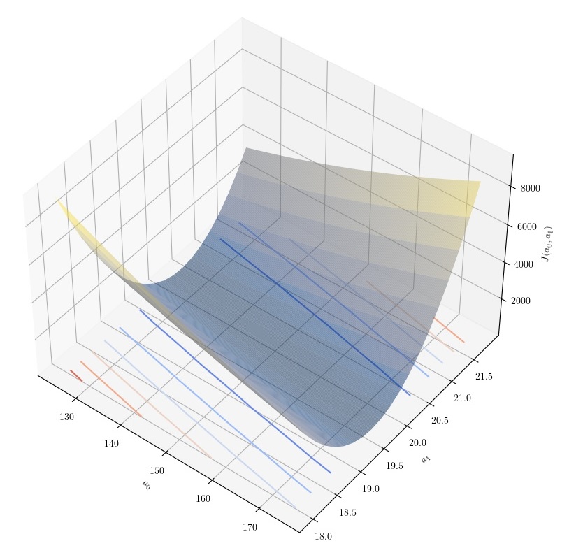
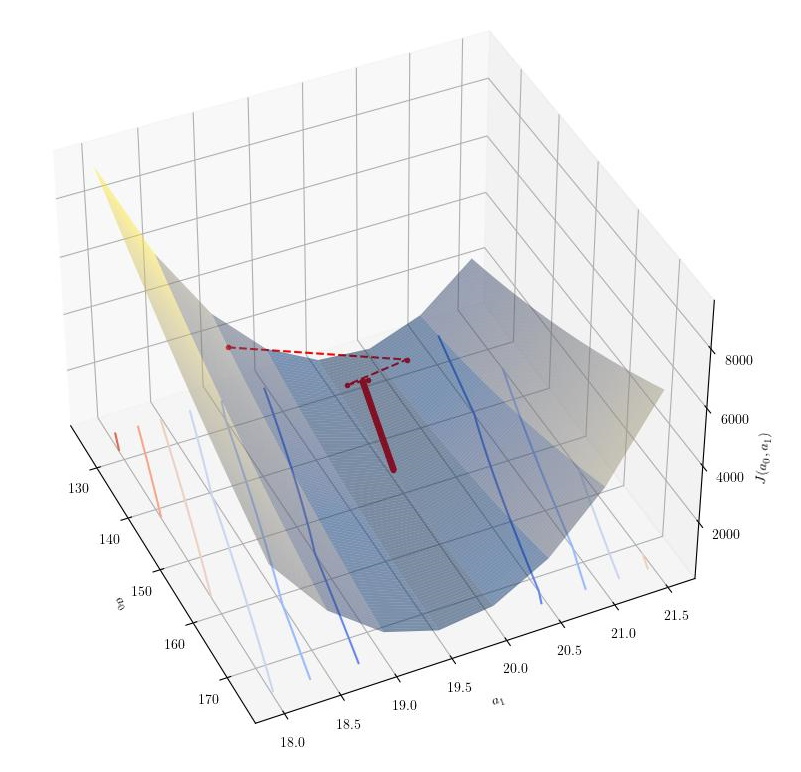
For the function $y = 150 + 20x + \xi $ the following plot was obtained.
 |
|---|
| Generation of univariate training set from $y = 150 + 20x + \xi $ |
| - |
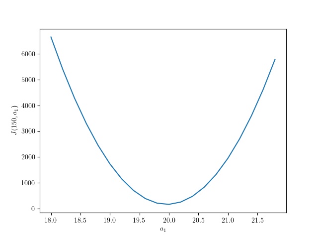
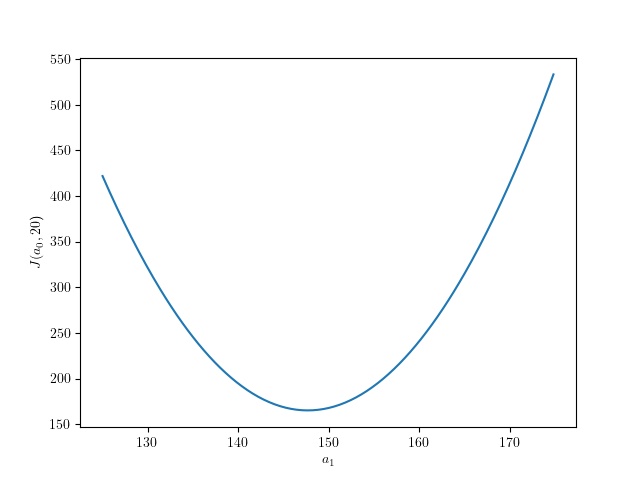
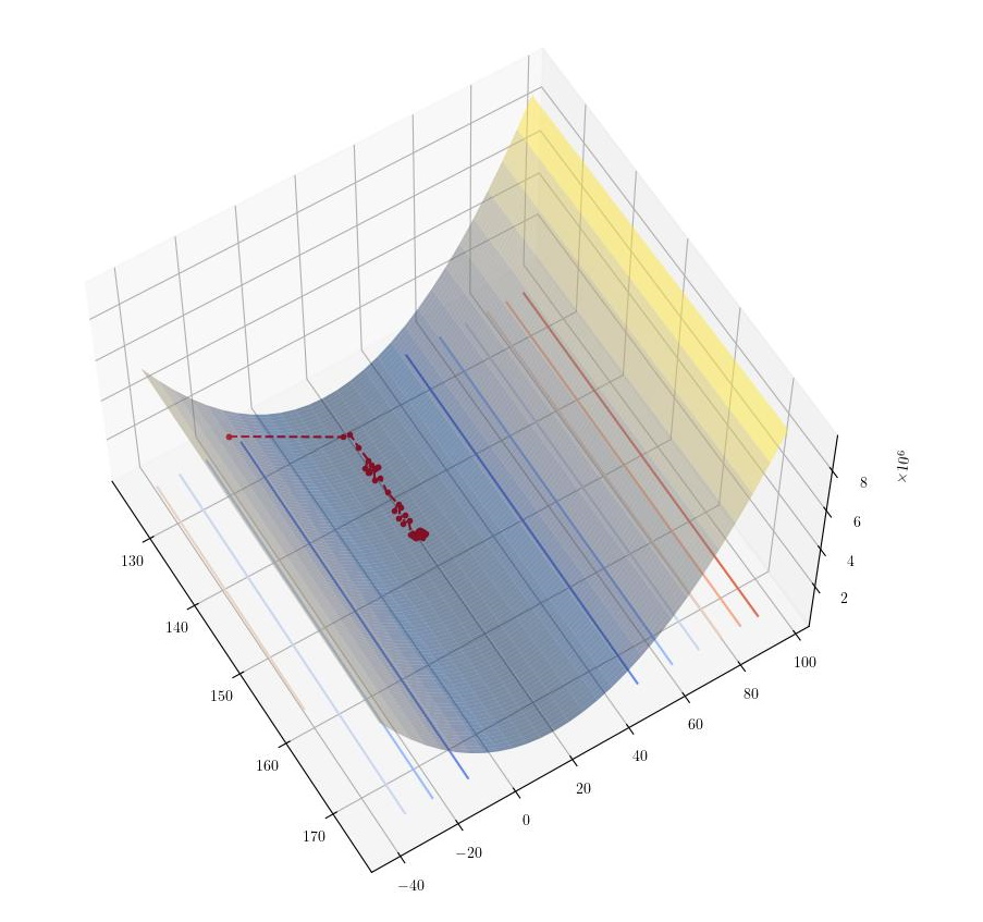
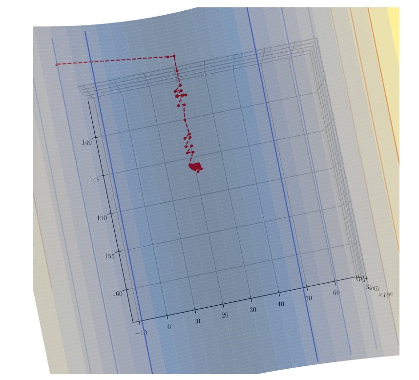
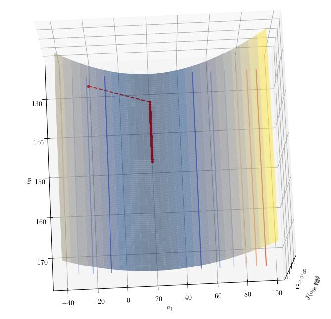
From this plot, it is not clear that the cost function has a single minimum. It is evident that the cost function has a minimum in the y ($a_1$) axis, but it is not visually obvious that the same is true for the x ($a_0$) axis. For this reason, we also plotted a slice of the cost function in the $a_0$ axis at $a_0 = 150$ and another slice at the $a_1$ axis at $a_1 = 20$. The plots are shown below.
 |
|---|
| Cost function slice at $a_0=150$ |
| - |
 |
|---|
| Cost function slice at $a_1=20$ |
| - |
We can conclude that the cost function does have a global minimum, but the rate of change in the $a_0$ axis is much lower than the rate of change in the $a_1$ axis. Therefore, we intuitively expect gradient descent to converge to the $a_1$ axis faster than the $a_0$ axis as the gradients in that axis are considerably larger.
Linear regression analysis
What is the best function that describes the data? In the linear regression post for the univariate case and multivariate case we have derived the function that can be used to fit the data. Using these functions on the data obtained from the generators can help us appreciate the effect of the random component of the data. It can also measure the accuracy of the techniques that we will use later on.
For the univariate case, $y = 150 + 20x + \xi $, the function obtained is the following: $$y = 147.075 + 20.012 x$$
For the multivariate case, $y = 12 + 5x_1 -3x_2 + \xi $, the function obtained is the following: $$y = 11.992 + 4.984 x_1 -2.998 x_2$$
Batch Gradient Descent
We then investigated the effect of gradient descent as an algorithm to minimize the cost function. In this phase, we had an opportunity to compare the performance difference between using vectorization and not. We have therefore implemented two versions of the gradient descent algorithm. As expected, using vectorization is much faster, around 50 times faster.
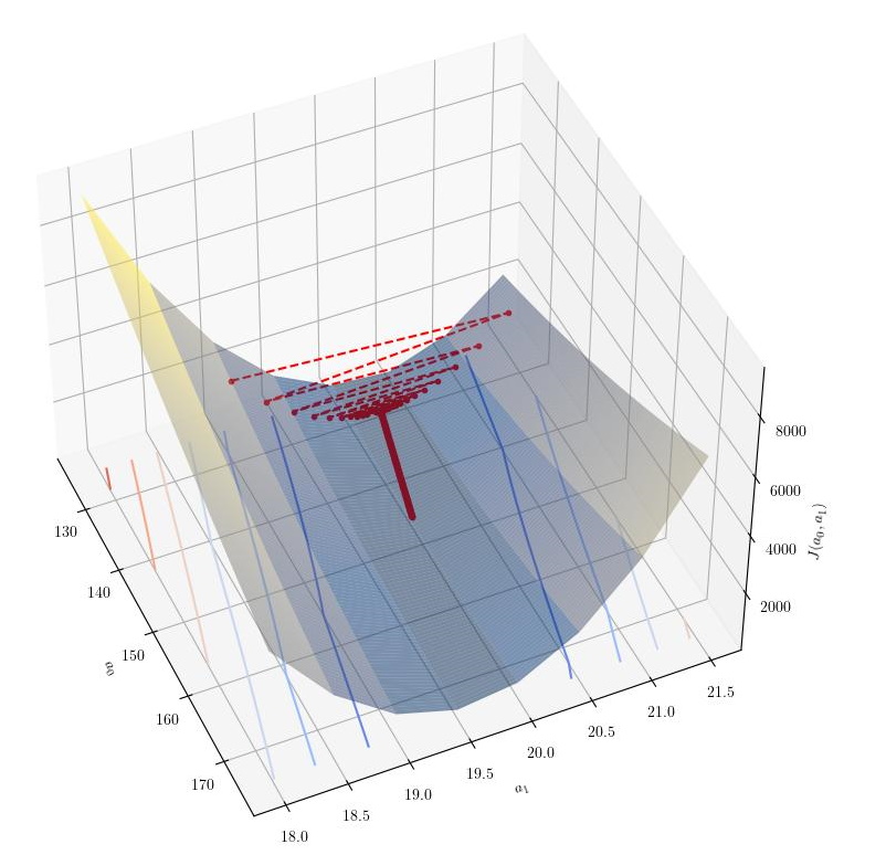
Thanks to the visualization developed previously; we also had an opportunity to see the effect of $\alpha$ on the algorithm. As expected, large $\alpha$ values oscillate in the execution, especially when moving down the $a_1$ axis, where the gradient is steeper. The following graphs show the effect of two values of $\alpha$ on the algorithm.
 |
|---|
| Batch Gradient descent with $\alpha=0.00056$ |
| - |
 |
|---|
| Batch Gradient descent with $\alpha=0.0004$ |
| - |
The results of the two functions batch gradient descent are shown below.
no-vectorization
$a_0$ : 11.7278
$a_1$ : 4.9834
$a_2$ : -2.9898
$J(a_0, a_1, a_2)$ : 12.8490
Epochs to converge : 5739
Execution time : 23.662
vectorization
$a_0$ : 11.7278
$a_1$ : 4.9834
$a_2$ : -2.9898
$J(a_0, a_1, a_2)$ : 12.8490
Epochs to converge : 5739
Execution time : 0.6546
The benefits of using vectorization are obvious
Stochastic Gradient Descent
As seen in theStochastic Gradient Descent post, the coefficients are updated after each training example is evaluated. Therefore, the result is a convergence to the minimum that does not necessarily improve the cost after each training example. The following graphs show the descent obtained with the stochastic gradient descent algorithm.
 |
|---|
| Stochastic Gradient Descent |
| - |
 |
|---|
| Stochastic Gradient Descent |
| - |
We implemented two stochastic gradient descent functions. The first one exists after a preset number of iterations are reached.
The second utilizes a validation set to determine if the algorithm has converged. The cost function is evaluated on the validation set, and the algorithm is stopped if the cost function converges.
One important consideration is that the benefits of vectorization are entirely lost in the stochastic gradient descent algorithm as we are evaluating one training example at a time.
The results of the stochastic gradient descent are shown below.
Fixed-iterations Exit (10 epochs)
$a_0$ : 11.4043
$a_1$ : 4.9771
$a_2$ : -2.9735
$J(a_0, a_1, a_2)$ : 12.90175
Epochs to converge : 10
Execution time : 1.6228
Use of Validation Set
$a_0$ : 11.9018
$a_1$ : 4.9691
$a_2$ : -2.9735
$J(a_0, a_1, a_2)$ : 12.8617
Epochs to converge : 100
Execution time : 12.0777
Mini-Batch Gradient Descent
The final investigation that was performed was the mini-batch gradient descent algorithm. Mini-batch gradient descent is a variant of stochastic gradient descent that uses a subset of the training set to update the coefficients. Hence, the coefficients are updated more frequently (after each mini-batch) whilst still maintaining some of the advantages of vectorization that were lost in the stochastic gradient descent algorithm.
The analysis plots show the results of the mini-batch gradient descent algorithm.
 |
|---|
| Mini-batch Gradient Descent |
| - |
We implemented two mini-batch gradient descent variants as we did to the stochastic gradient descent. The first one exists after a preset number of iterations is reached, whilst the second one utilizes a validation set to determine if the algorithm has converged. The cost function is evaluated on the validation set, and the algorithm is stopped if the cost function converges.
The results of the mini-batch gradient descent are shown below.
Fixed-iterations Exit
$a_0$ : 11.7030
$a_1$ : 4.9852
$a_2$ : -2.9912
$J(a_0, a_1, a_2)$ : 12.85275
Mini-batches to converge : 1000
Execution time : 1.2512
Validation Set
$a_0$ : 11.8963
$a_1$ : 4.9850
$a_2$ : -2.9965
$J(a_0, a_1, a_2)$ : 12.8440
Mini-batches to converge : 1320
Execution time : 1.5632
Conclusion
This series investigated several techniques to solve the linear regression problem. We investigated batch gradient descent, stochastic gradient descent, and mini-batch gradient descent. The analysis results were then presented in the form of graphs and tables..