We have discussed the multivariate linear regression problem in the previous posts, and we have seen that in this case the hypothesis function becomes:

$$\hat{y} = a_0 + a_1 x_1 + a_2 x_2 + \dots + a_n x_n$$

If we define $x_0$, such that $x_0 = 1$, then the hypothesis function becomes:

$$\hat{y} = a_0 x_0 + a_1 x_1 + a_2 x_2 + \dots + a_n x_n$$

Let us now consider a dataset of $m$ points. we can therefore calculate the hypothesis function for each point,

$$\hat{y}^{(1)} = a_0 x_0^{(1)} + a_1 x_1^{(1)} + a_2 x_2^{(1)} + \dots + a_n x_n^{(1)}$$

$$\hat{y}^{(2)} = a_0 x_0^{(2)} + a_1 x_1^{(2)} + a_2 x_2^{(2)} + \dots + a_n x_n^{(2)}$$

$$\dots$$

$$\hat{y}^{(m)} = a_0 x_0^{(m)} + a_1 x_1^{(m)} + a_2 x_2^{(m)} + \dots + a_n x_n^{(m)}$$

where $x_1^{(i)}$ is the first feature of the $i$th point and,

$x_0^i = 1 \forall i$.

we can express the equation of the hypothesis function shown above as a matrix multiplication. Let us start by defining the matrix $X$ as the matrix of features, such that;

$$\textbf{X} = \begin{pmatrix} x_0^{(1)} & x_0^{(2)} & \dots & x_0^{(m)} \\
x_1^{(1)} & x_1^{(2)} & \dots & x_1^{(m)} \\
\vdots & \vdots & \vdots & \vdots \\
x_n^{(1)} & x_n^{(2)} & \dots & x_n^{(m)} \end{pmatrix}$$ $$Dim:[n \times m]$$

where, for example, $x^{(2)}$ or the second feature point,

$$x^{(2)} = \begin{pmatrix} x_0^{(2)} \\
x_1^{(2)} \\
\vdots \\
x_n^{(2)} \end{pmatrix}$$ $$Dim:[n \times 1]$$

the matrix of coefficients $\beta$ as:

$$\beta = \begin{pmatrix} a_0 \\
a_1 \\
\vdots \\
a_n \end{pmatrix}$$ $$Dim:[n \times 1]$$

and the matrix of predictions $\hat{Y}$ as:

$$\hat{Y} = \begin{pmatrix} \hat{y}^{(1)} \\
\hat{y}^{(2)} \\
\vdots \\
\hat{y}^{(m)} \end{pmatrix}$$ $$Dim:[n \times 1]$$

We can now calculate the hypothesis function as a matrix multiplication:

$$\begin{pmatrix} \hat{y}^{(1)} \\
\hat{y}^{(2)} \\
\vdots \\
\hat{y}^{(m)} \end{pmatrix} = \begin{pmatrix} x_0^{(1)} & x_1^{(1)} & \dots & x_n^{(1)} \\
x_0^{(2)} & x_1^{(2)} & \dots & x_n^{(2)} \\
\vdots & \vdots & \vdots & \vdots \\
x_0^{(m)} & x_1^{(m)} & \dots & x_n^{(m)} \end{pmatrix} \begin{pmatrix} a_0 \\
a_1 \\
\vdots \\
a_n \end{pmatrix} $$ $$Dim:[m \times n] \cdot [n \times 1]$$ or

$$\hat{Y} = X^{T} \cdot \beta$$

We can now define the matrix of residuals as:

$$\textbf{R} = \begin{pmatrix} \hat{y}^{(1)} \\
\hat{y}^{(2)} \\
\vdots \\
\hat{y}^{(m)} \end{pmatrix} - \begin{pmatrix} y^{(1)} \\
y^{(2)} \\
\vdots \\
y^{(m)} \end{pmatrix} = \begin{pmatrix} \hat{y}^1 - {y}^1 \\
\hat{y}^2 - {y}^2 \\
\vdots \\
\hat{y}^m - {y}^m \end{pmatrix}$$

we can therefore update the coefficients $\beta$ as:

$$\begin{pmatrix} a_0 \\
a_1 \\
\vdots \\
a_n \end{pmatrix} := \begin{pmatrix} a_0 \\
a_1 \\
\vdots \\
a_n \end{pmatrix} - \frac{\alpha}{m} \begin{pmatrix} x_0^{(1)} & x_0^{(2)} & \dots & x_0^{(m)} \\
x_1^{(1)} & x_1^{(2)} & \dots & x_1^{(m)} \\
\vdots & \vdots & \vdots & \vdots \\
x_n^{(1)} & x_n^{(2)} & \dots & x_n^{(m)} \end{pmatrix} \cdot \begin{pmatrix} \hat{y}^1 - {y}^1 \\
\hat{y}^2 - {y}^2 \\
\vdots \\
\hat{y}^m - {y}^m \end{pmatrix}$$ $$Dims: [n \times m] \cdot [m \times 1]$$ or

$$\beta := \beta - \frac{\alpha}{m} \textbf{X} \cdot \textbf{R}$$

The cost function, $J$, which was defined in the previous post as:

$$J = \frac{1}{2m} \sum_{i=1}^m \left( \hat{y}^{(i)} - {y}^{(i)} \right)^2$$

can be obtained as:

$$ J(\beta) = \frac{1}{2m} \beta^T \cdot \beta$$

The full python code for this algorithm can be seen below. Numpy is used for the matrix operations, and the equations above are actually implemented in just the following four lines of code.

  self.__y_hat = np.dot(self.__beta, self.__X.T)

  #  calculate the residuals
  residuals = self.__y_hat - self.__y
  
  # calculate the new value of beta
  self.__beta -= (self.__alpha/self.__m) * np.dot(residuals, self.__X)

  # calculate the cost function
  cost = np.dot(residuals, residuals)/(2 * self.__m)

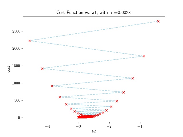
In the example, the code plots the cost function as a function of $a_2$. We notice convergence is achieved after 6676 iterations for a reasonably large value of $\alpha$.

import os
import matplotlib
matplotlib.rcParams['text.usetex'] = True
import matplotlib.pyplot as plt
import pandas as pd
import sys
import numpy as np


def multifeature_gradient_descent(file, alpha=0.0023, threshold_iterations=100000, costdifference_threshold=0.00001, plot=False):

    X = None
    Y = None
    beta = None

    full_filename = os.path.join(os.path.dirname(__file__), file)
    training_data = pd.read_csv(full_filename, delimiter=',', header=0, index_col=False)

    Y = training_data['y'].to_numpy()
    
    m = len(Y)

    X = training_data.drop(['y'], axis=1).to_numpy()
    
    # add a column of ones to the X matrix to account for the intercept, a0
    X = np.insert(X, 0, 1, axis=1)
    print(X)
    
    y_hat = np.zeros(len(Y))
    
    # beta will hold the values of the coefficients, hence it will be  the size 
    # of a row of the X matrix
    beta = np.random.random(len(X[0]))

    iterations = 0

    # initialize the previous cost function value to a large number
    previous_cost = sys.float_info.max
    
    # store the cost function and a2 values for plotting
    costs = []
    a_2s = []
    
    while True:
        # calculate the hypothesis function for all training data
        y_hat = np.dot(beta, X.T)

        #  calculate the residuals
        residuals = y_hat - Y
        
        # calculate the new value of beta
        beta -= (alpha/m) * np.dot(residuals, X)

        # calculate the cost function
        cost = np.dot(residuals, residuals)/(2 * m)

        # increase the number of iterations
        iterations += 1

        # record the cost and a1 values for plotting
        costs.append(cost)
        a_2s.append(beta[2])
        
        cost_difference = previous_cost - cost
        print(f'Epoch: {iterations}, cost: {cost:.3f}, beta: {beta}')
        previous_cost = cost

        # check if the cost function is diverging, if so, break
        if cost_difference < 0:
            print(f'Cost function is diverging. Stopping training.')
            break
        
        # check if the cost function is close enough to 0, if so, break or if the number of 
        # iterations is greater than the threshold, break
        if abs(cost_difference) < costdifference_threshold or iterations > threshold_iterations:
            break
    
    if plot:
        # plot the cost function and a1 values
        plt.plot(a_2s[3:], costs[3:], '--bx', color='lightblue', mec='red')
        plt.xlabel('a2')
        plt.ylabel('cost')
        plt.title(r'Cost Function vs. a1, with $\alpha$ =' + str(alpha))
        plt.show()

    return beta

if __name__ == '__main__':
    
    file = 'data.csv'
    alpha = 0.0023
    threshold_iterations = 100000
    costdifference_threshold = 0.00001
    plot = False

    beta = multifeature_gradient_descent(file, alpha, threshold_iterations, costdifference_threshold, plot)
    print(f'Final beta: {beta}')