In this post we will implement the multivariate linear regression model for 2 features in python. We gave already seen in the last post, that for this case, $a_0$, $a_1$ and $a_2$ can be solved by;

$$a_1 = \frac{ \sum_{i=1}^{n} X_{2i}^2 \sum_{i=1}^{n} X_{1i}y_i - \sum_{i=1}^{n} X_{1i}X_{2i} \sum_{i=1}^{n} X_{2i}y_i } {\sum_{i=1}^{n}X_{1i}^2 \sum_{i=1}^{n}X_{2i}^2 - (\sum_{i=1}^{n} X_{1i}X_{2i})^2}$$

$$a_2 = \frac{ \sum_{i=1}^{n} X_{1i}^2 \sum_{i=1}^{n} X_{2i}y_i - \sum_{i=1}^{n} X_{1i}x_{2i} \sum_{i=1}^{n} X_{1i}y_i } {\sum_{i=1}^{n}X_{1i}^2 \sum_{i=1}^{n}X_{2i}^2 - (\sum_{i=1}^{n} X_{1i}X_{2i})^2}$$

and

$$ a_0 = \bar{\textbf{Y}} - a_1 \bar{\textbf{X}}_1 - a_2 \bar{\textbf{X}}_2$$

where $$ \sum_{i=1}^{n} X_{1i}^2 = \sum_{i=1}^{n} x_{1i}^2 - \frac{\sum_{i=1}^{n} x_{1i}^2}{n}$$

$$ \sum_{i=1}^{n} X_{1i}^2 = \sum_{i=1}^{n} x_{1i}^2 - \frac{\sum_{i=1}^{n} x_{1i}^2}{n}$$

$$ \sum_{i=1}^{n} X_{1i}y_{i} = \sum_{i=1}^{n} x_{1i} \sum_{i=1}^{n} y_{i} - \frac{\sum_{i=1}^{n} x_{1i} \sum_{i=1}^{n} y_{i}}{n}$$

$$ \sum_{i=1}^{n} X_{2i}y_{i} = \sum_{i=1}^{n} x_{2i} \sum_{i=1}^{n} y_{i} - \frac{\sum_{i=1}^{n} x_{2i} \sum_{i=1}^{n} y_{i}}{n}$$

$$ \sum_{i=1}^{n} X_{1i}X_{2i} = \sum_{i=1}^{n} x_{1i} \sum_{i=1}^{n} x_{2i} - \frac{\sum_{i=1}^{n} x_{1i} \sum_{i=1}^{n} x_{2i}}{n}$$

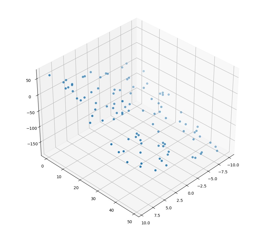
We will start this test by generating a dataset with 2 features and a linear relationship between them. the equation used in this case is:

$$y = 12 + 5x_1 -3x_2$$

The dataset will be generated with the following procedure:

• Generate the points according to the equation above
• Add noise to the points
• sample 1% of the points for testing

This is accomplished by the following code:

import matplotlib.pyplot as plt
import numpy as np
import pandas as pd

fig = plt.figure(figsize=(12, 12))
ax = fig.add_subplot(projection='3d')

x1_lower = -10
x1_higher = 10
x1_step = (x1_higher - x1_lower) / 100
x1 = np.arange(x1_lower, x1_higher, x1_step)

x2_lower = 0
x2_higher = 50
x2_step = (x2_higher - x2_lower) / 100
x2= np.arange(x2_lower, x2_higher, x2_step)

# generate the plane
xx1, xx2 = np.meshgrid(x1, x2)
y = 12 + (5 * xx1) + (-3 * xx2)

# add random_multiplier to y
random_multiplier = 5
e = np.random.randn(len(xx1), len(xx2) )*random_multiplier
yy = y + e


df = pd.DataFrame(data=[xx1.ravel(), xx2.ravel(), yy.ravel()]).T
df = df.sample(frac=0.01)
df.columns = ['x1', 'x2', 'y']
df.to_csv("data.csv", header=True, index=False)

# plot the data
y = df.iloc[:,1]
x = df.iloc[:,0]
z = df.iloc[:,2]
ax.scatter(x,y,z, cmap='coolwarm')
plt.show()

A visualization of the data is shown in the figure below.

The implementation of the regression algorithm for this case is as follows:

import pandas as pd

# import data from csv
data = pd.read_csv("data.csv")

data['x1_sq'] = data['x1']**2
data['x2_sq'] = data['x2']**2
data['x1y'] = data['x1']*data['y']
data['x2y'] = data['x2']*data['y']
data['x1x2'] = data['x1']*data['x2']

n = len(data)

sum_X1_sq = data['x1_sq'].sum() - (data['x1'].sum()**2)/n
print(f'sum_X1_sq: {sum_X1_sq}')

sum_X2_sq = data['x2_sq'].sum() - (data['x2'].sum()**2)/n
print(f'sum_x2_sq: {sum_X2_sq}')

sum_X1y = data['x1y'].sum() - (data['x1'].sum()*data['y'].sum())/n
print(f'sum_X1y: {sum_X1y}')

sum_X2y = data['x2y'].sum() - (data['x2'].sum()*data['y'].sum())/n
print(f'sum_X2y: {sum_X2y}')

sum_X1X2 = data['x1x2'].sum() - (data['x1'].sum()*data['x2'].sum())/n
print(f'sum_X1X2: {sum_X1X2}')

mean_y = data['y'].mean()
mean_x1 = data['x1'].mean()
mean_x2 = data['x2'].mean()

n = len(data)

a1 = (sum_X2_sq*sum_X1y - sum_X1X2*sum_X2y)/(sum_X1_sq*sum_X2_sq - sum_X1X2**2)

a2 = (sum_X1_sq*sum_X2y - sum_X1X2*sum_X1y)/(sum_X1_sq*sum_X2_sq - sum_X1X2**2)

a0 = mean_y - a1*mean_x1 - a2*mean_x2

print(f'a0: {a0}, a1: {a1}, a2: {a2}')

The results obtained are; $a_0: 11.511, a_1: 5.029, a2: -2.992$. Close enough when considering the noise in the data and that we only used a very small portion of the data for the test.

Conclusion

It is important to note that there was an explosion in the number of calculations required to solve this problem when compared to the univariate case, so we can conclude that solving this problem with this method for more features will be prohibitively computationally expensive. An approximation that will give reasonably close results will be discussed in a future post.