Logistic regression is a machine learning algorithm that is commonly used for binary classification tasks.
Given a feature vector X∈Rnx, the goal of logistic regression is to predict the probability ˆy that a binary output variable y takes the value 1, given X, that is ˆy=P(y=1|X), 0≤y≤1. For example, in the case of image classification, logistic regression can be used to predict the probability that an image contains a cat.
 |
||
|---|---|---|
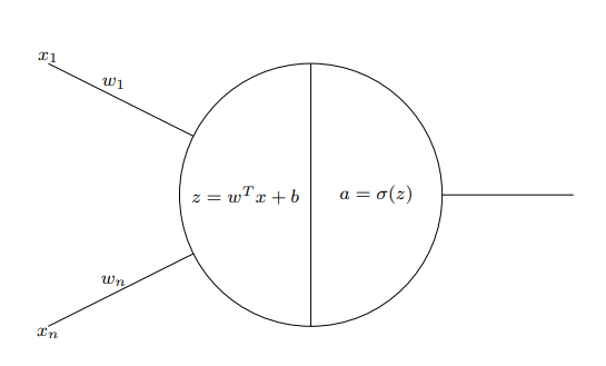
The logistic regression model consists of three main components:
- Parameters: A weight vector ω∈Rnx and a bias term b∈R.
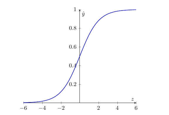
- Sigmoid function: A function σ(z)=11+e−z, which maps any real number z to the range (0,1). This function is used to ensure that the predicted probability ˆy is always between 0 and 1.
- Output: The predicted probability ˆy is computed as ˆy=σ(ωTX+b).
The weight vector ω and the bias term b are learned from a labelled training set by minimizing a suitable loss function using techniques such as gradient descent or its variants. Once trained, the logistic regression model can be used to predict the probability of the binary output variable for new input examples.
 |
||
|---|---|---|
The feedforward process for logistic regression can be described as follows:
- Compute z as the dot product of the weight vector ω and the input features, plus the bias term b: z=ωTx+b
- Pass z through the sigmoid function to obtain the predicted output ˆy: ˆy=σ(z)=11+e−z
- Define the loss function L as the negative log-likelihood of the predicted output given the true label: L=−(ylog(ˆy)+(1−y)log(1−ˆy))To optimize the weight vector ω, one common method is to compute the derivatives of the loss function with respect to each weight and the bias term, and use these derivatives to update the weights in the opposite direction of the gradient. This is known as gradient descent.
To compute the derivatives, we use the chain rule of derivatives:
∂L∂ωi=∂L∂ˆy⋅∂ˆy∂z⋅∂z∂ωi
∂L∂b=∂L∂ˆy⋅∂ˆy∂z⋅∂z∂b
We can then use these derivatives to update the weights as follows:
ωi←ωi−α∂L∂ωi
and
b←b−α∂L∂b
Where α is the learning rate, which controls the step size of the updates. By iteratively performing these updates on a training set, we can find the optimal weight vector ω that minimizes the loss function on the training set.
The Derivatives
Let’s begin by computing the derivative of the loss function with respect to the predicted output ˆy: ∂L∂ˆy=∂∂ˆy(−(ylog(ˆy)+(1−y)log(1−ˆy)))
Using the chain rule, we get:
∂L∂ˆy=−yˆy+1−y1−ˆy
The derivative of the predicted output ˆy with respect to z:
∂ˆy∂z=∂∂zσ(z)=∂∂z11+e−z
Using the quotient rule, we get: ∂ˆy∂z=e−z(1+e−z)2=11+e−z⋅e−z1+e−z=ˆy(1−ˆy)
The derivative of z with respect to ωi: ∂z∂ωi=∂∂ωiωTx+b=∂∂ωi(ω1x1+⋯+wixi+⋯+wnxn)+b=xi
Similarly, ∂z∂b=∂∂bωTx+b=∂∂b(ω1x1+⋯+wixi+⋯+wnxn)+b=1
Therefore
∂L∂ωi=∂L∂ˆy⋅∂ˆy∂z⋅∂z∂ωi=(−yˆy+1−y1−ˆy)⋅(ˆy(1−ˆy))⋅(xi)=(ˆy−y)xi
and
∂L∂b=∂L∂ˆy⋅∂ˆy∂z⋅∂z∂b=(−yˆy+1−y1−ˆy)⋅(ˆy(1−ˆy))⋅(1)=(ˆy−y)
Extreme Cases
When the predicted value is 1, i.e., ˆy=1, the derivative of the loss with respect to the predicted output, ∂L∂ˆy, will be undefined because of the term 1−y1−ˆy in the equation.
Similarly, in the case where the predicted value is exactly 0, i.e., ˆy=0, the derivative of the loss with respect to the predicted output, ∂L∂ˆy, will also be undefined because of the term −yˆy in the equation.
In these cases, the backpropagation step cannot proceed as usual, since the derivative of the loss function with respect to the predicted output is a required component. One approach to address this issue is to add a small value ϵ to ˆy in the calculation of the loss function, so that the logarithm term is well-defined. This is sometimes called “label smoothing”.
Another approach is to use a modified loss function that does not have this issue, such as the hinge loss used in support vector machines (SVMs). However, it’s worth noting that logistic regression is a popular and effective method for binary classification, and the issue of undefined derivatives is relatively rare in practice.