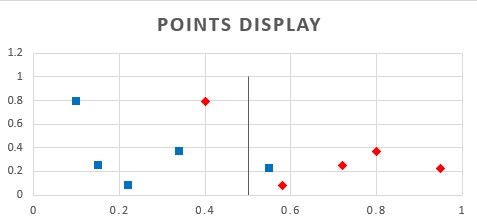
A binary classifier is a function that can be applied to features X to produce a Y value of true (1) or false (0). It is a supervised learning technique; therefore, a test set is extracted from the available data so that the model is validated before deployed in production.

$$ f(x_1, x_2, x_3, \dots, x_n) = Y \in {0, 1} $$

The function will return a value between 0 and 1, and a threshold value is therefore operated to classify the result as a true or false. The model will subsequently classify predictions as true or false according to the threshold value.

Given the above, we can obtain four kinds of results:

• A prediction of 1 for an observation that has a label value of 1, This is known as True Positive (TP)
• A prediction of 1 for an observation that has a label value of 0, This is known as False Positive (FP)
• A prediction of 0 for an observation that has a label value of 0, This is known as True Negative(TN)
• A prediction of 0 for an observation that has a label value of 1, This is known as False Negative(FN)

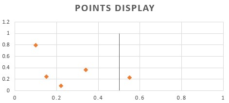
An excel sheet has been created to demonstrate these basic concepts. The example in the sheet defines five true and five false samples that are displayed in a graph. A threshold value can be set to determine the TP, TN, FP and FN samples.

The number of samples that are TP, TN, FP or FN can be organized in what is known as a confusion matrix. This tool makes it easy to perform calculations that determine the validity of the model at hand.

Accuracy

The accuracy of the model can be defined as the number of samples that were correctly classified divided by the total number of samples, hence,

$$Accuracy=\frac{TP+TN}{TP+FP+TN+FN}$$

Whilst testing using accuracy can be used in some situations, it has a severe flaw that makes it unsuitable in others. In particular, when the number of TN is much greater than TP or vice versa, this measure will always produce a very high result. A typical such scenario when the model at hand is detecting anomalies, for example, tumours from a scanned image.

Precision

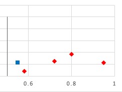
A more robust metric is the precision or the ratio of the TP from all the samples classified as true. We, therefore, consider only the positive side of our diagram to obtain this metric:

$$Precision=\frac{TP}{TP+FP}$$

Receiver Operator Characteristic (ROC)

Two other metrics that can be used are the True Positive Rate (TPR) and the False Positive Rate (FPR). The TPR is the ratio of the correctly classified true samples (TP) and the total number of true samples, (TP and FN), hence,

$$TPR =\frac{TP}{TP+FN}$$

Conversely, the false positive rate (FPR) is the ratio of the samples incorrectly classified as true (FP) and the total number of false samples (TF and FP), hence.

$$FPR = \frac{FP}{FP+TN}$$

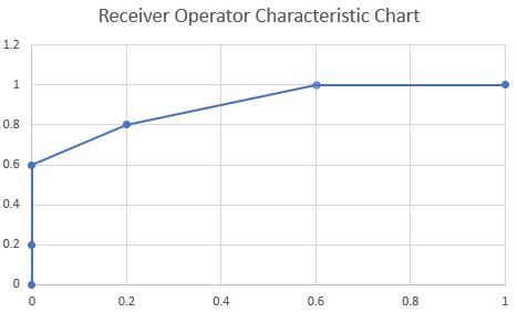
Intuitively we can determine that different values of TPR and FPR are obtained as the threshold value is varied. The (FPR, TPR) pairs obtained for each threshold value can be plotted on what is known as the Receiver Operator Characteristic (ROC) chart.

The area under the ROC chart is an indicator of the prediction accuracy of the model. The objective of a model is for the ROC curve to reach a TPR value of 1 for the smallest possible value of FPR. Therefore the largest possible area of the ROC curve is the area of a square having sides of 1 and is therefore 1.