This post will look at Interval Type-2 fuzzy set (IT2FS) and its reduction. We have already discussed the basics of Type-2 fuzzy sets in a previous post, and we have seen that a general type-2 fuzzy set can be defined as follows:

$$\tilde{A}=\int_{x\in X}\int_{u\in J_{x}} \mu_{\tilde{A}}(x,u) / (x,u)$$

where $J_{x}\subseteq[0,1]$

And if, as an example, we consider the following general type-2 fuzzy set:

(1.0/0 + 0.5/0.2 + 0.3/0.4 + 0.1/0.6                       )/1+
(0.5/0 + 1.0/0.2 + 0.5/0.4 + 0.3/0.6 + 0.1/0.8             )/2+
(0.1/0 + 0.3/0.2 + 0.5/0.4 + 1.0/0.6 + 0.5/0.8 + 0.3/1.0   )/3+
(        0.1/0.2 + 0.3/0.4 + 0.5/0.6 + 1.0/0.8 + 0.5/1.0   )/4+
(1.0/0 + 0.5/0.2 + 0.3/0.4 + 0.1/0.6                       )/5

The set can be created and displayed using the type2fuzzy library as follows:

from type2fuzzy import GeneralType2FuzzySet
from type2fuzzy.display.generaltype2fuzzysetplot import GeneralType2FuzzySetPlot
import matplotlib.pyplot as plt

# Create a general type-2 fuzzy set
gt2fs_rep =   '''
 (1.0/0 + 0.5/0.2 + 0.3/0.4 + 0.1/0.6                       )/1
+(0.5/0 + 1.0/0.2 + 0.5/0.4 + 0.3/0.6 + 0.1/0.8             )/2
+(0.1/0 + 0.3/0.2 + 0.5/0.4 + 1.0/0.6 + 0.5/0.8 + 0.3/1.0   )/3
+(        0.1/0.2 + 0.3/0.4 + 0.5/0.6 + 1.0/0.8 + 0.5/1.0   )/4
+(1.0/0 + 0.5/0.2 + 0.3/0.4 + 0.1/0.6                       )/5'''

gt2fs = GeneralType2FuzzySet.from_representation(gt2fs_rep)

# Plot the general type-2 fuzzy set
print(f'\nSet representation: {gt2fs}')

fig = plt.figure()
ax=fig.add_subplot(1,1,1)

set_plt = GeneralType2FuzzySetPlot(gt2fs)
set_plt.plot(ax)

plt.show()

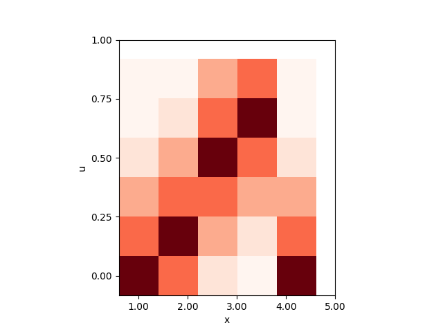
which will result in the following plot:

Interval Type-2 fuzzy set (IT2FS)

An Interval Type-2 Fuzzy set (IT2FS) is a Type-2 fuzzy set where all the secondary grades are equal to 1. Therefore, secondary grades have no information; hence, we can describe the set by their Footprint of uncertainty and thus by their Lower and upper membership functions. Accordingly, an IT2FS is defined as follows:

$$C_{\tilde{A}} = \int_{\theta_{1}\in J_{x_{1}}} \dots \int_{\theta_{N}\in J_{x_{N}}} 1 / \frac{\sum_{i=1}^{N} x_i \theta_{i}}{\sum_{i=1}^{N} \theta_{i}}$$

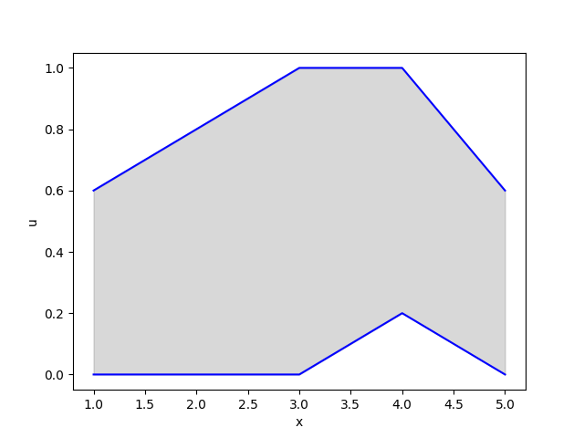
we can see by inspection that the IT2FS equivalent of the general tye-2 fuzzy set under examination is the following:

[0.00000, 0.60000]/1.0+
[0.00000, 0.80000]/2.0+
[0.00000, 1.00000]/3.0+
[0.20000, 1.00000]/4.0+
[0.00000, 0.60000]/5.0

We can obtain an instance of this set by using the type2fuzzy library as follows:

from type2fuzzy import IntervalType2FuzzySet
from type2fuzzy.display.intervaltype2fuzzysetplot import IntervalType2FuzzySetPlot

it2fs = IntervalType2FuzzySet.from_general_type2_set(gt2fs)

print(f'\nSet representation: {it2fs}')

fig = plt.figure()
ax=fig.add_subplot(1,1,1)

set_plt = IntervalType2FuzzySetPlot(it2fs)
set_plt.plot(ax)

plt.show()

which will plot the following:

Centroid of an Interval Type-2 fuzzy set

An iterative procedure to find the Centroid of an Interval Type-2 fuzzy is discussed in

“Karnik, N. N., & Mendel, J. M. (1998, May). Introduction to type-2 fuzzy logic systems. In 1998 IEEE international conference on fuzzy systems proceedings. IEEE world congress on computational intelligence (Cat. No. 98CH36228) (Vol. 2, pp. 915-920). IEEE."

Which addresses the following problem:

Given $x_i \in \Re$ where ${i = 1, \dots, N} $ and $\omega_i \equiv \Omega_i \in [ \bar{\omega_i}, \overline{\omega_i} ]$ where ${i = 1, \dots, N} $

such that

$\underline{\omega_i} \leq \bar{\omega_i}$ for all ${i = 1, \dots, N} $

we want to find

$$Y = \frac{\sum_{i=1}^{N} x_i \Omega_i}{\sum_{i=1}^{N} \Omega_i} \equiv [y_l, y_r]$$

where

$$y_r \equiv \min_{x_i \in \Re, \forall i ; \omega_i \in [ \bar{\omega_i}, \overline{\omega_i} ], \forall i } \frac{\sum_{i=1}^{N} x_i \omega_i}{\sum_{i=1}^{N} \omega_i} $$

and

$$y_l \equiv \max_{x_i \in \Re, \forall i ; \omega_i \in [ \bar{\omega_i}, \overline{\omega_i} ], \forall i } \underline{x_2} $$

The original Karnik Mendel algorithm is as follows:

1. Sort $x_i$, $(i=1, \dots, N)$ such that $\underline{x_1} \leq \underline{x_2} \leq \dots \leq\underline{x_N} $ . Ensure that $\omega_i$ remains matched to $x_i$.

2. Initialize $$\omega_i = \frac{\underline{\omega_1} + \overline{\omega_i}}{2}$$ and compute$$ y = \frac{\sum_{i=1}^{N} x_i \omega_i}{\sum_{i=1}^{N} \omega_i}$$

3. Find the switch point $k$, where $x_k \leq y$ and $x_{k} \leq y \leq x_{k+1}$

4. To find $y_l$		To find $y_r$
   set $\omega_i = \overline{\omega_i}$ for $i \leq k$		set $\omega_i = \underline{\omega_i}$ for $i \leq k$
   set $\omega_i = \underline{\omega_i}$ for $i > k$		set $\omega_i = \overline{\omega_i}$ for $i > k$

5. Compute $$ y' = \frac{\sum_{i=1}^{N} x_i \omega_i}{\sum_{i=1}^{N} \omega_i}$$

6. Evaluate;

   • If $|y'-y| \leq \xi$
     • STOP

     • For $y_l$		For $y_r$
       $y_l = y'$		$y_r = y'$

   • If $ |y'-y | > \xi$
     • Go to step 3

Implementation of IT2FS Type Reduction Algorithm

We implemented the above algorithm in the type2fuzzy library following function:

def _it2_kernikmendel_reduce_noinfo(it2fs, precision=5):

    numerator = 0
    denominator = 0
    error_threshold = 1e-5
    primary_domain_elements = it2fs.primary_domain()

    centroid = CrispSet(
        primary_domain_elements[0],
        primary_domain_elements[len(primary_domain_elements)-1])


    centroid_left = it2fs.mid_domain_element()
    while True:

        centroid.left = centroid_left
        numerator = 0
        denominator = 0

        for domain_element in it2fs.primary_domain():

            if domain_element >= centroid_left:
                numerator = numerator + (domain_element * it2fs[domain_element].left)
                denominator = denominator + it2fs[domain_element].left
            else:
                numerator = numerator + (domain_element * it2fs[domain_element].right)
                denominator = denominator + it2fs[domain_element].right

        if denominator == 0:
            centroid.left = it2fs.mid_domain_element()
            logging.log(logging.ERROR, 'error in calculating z_l, denominator is 0')
            break

        centroid_left = numerator / denominator

        if abs(centroid_left - centroid.left) <= error_threshold:
            break

To demonstrate the use of the above algorithm, we will use the example defined in the following paper.

Morales, Omar Salazar, José Humberto Serrano Devia, and José Jairo Soriano Méndez. “Centroid of an interval type-2 fuzzy set: Continuous vs. discrete.” Ingeniería 16.2 (2011): 67-78.

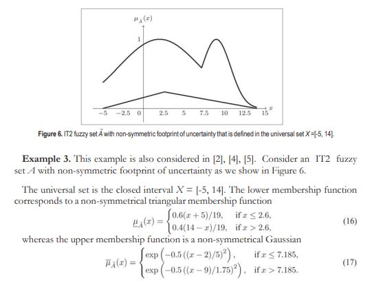
In this paper, Salazar et al. investigate the type-reduction of an IT2FS defined as follows:

We will therefore perform the following steps to replicate the above example:

• generate the IT2FS defined in the paper
• use the type2fuzzy library to find its Centroid

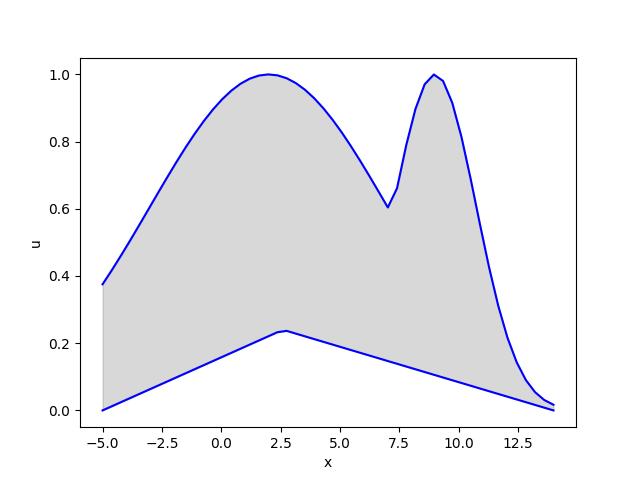
The following code will generate the IT2FS:

from math import exp
import numpy as np
import matplotlib.pyplot as plt
from type2fuzzy_library.membership.intervaltype2fuzzyset import IntervalType2FuzzySet
from type2fuzzy_library.display.intervaltype2fuzzysetplot import IntervalType2FuzzySetPlot
from type2fuzzy_library.type_reduction.it2_karnikmendel_reducer import it2_kernikmendel_reduce

X_LOW = -5
X_HIGH = 14
STEPS = 50

DELTA = (X_HIGH - X_LOW) / STEPS

lmv = lambda x: 0.6*(x+5)/19 if x <= 2.6 else 0.4*(14-x)/19
umv = lambda x: exp(-0.5*((x-2)/5)**2) if x <= 7.185 else exp(-0.5*((x-9)/1.75)**2)

it2fs = IntervalType2FuzzySet()

i =0
for x in np.linspace(X_LOW, X_HIGH, STEPS):
    it2fs.add_point(x, lmv(x), umv(x))

fig, ax = plt.subplots()
plot = IntervalType2FuzzySetPlot(it2fs)
plot.plot(ax)
plt.show()

We notice that we have also used the IntervalType2FuzzySetPlot class to plot the IT2FS. The following plot shows the IT2FS that we have generated:

Finally, we generate the Centroid of the IT2FS. Using the type2fuzzy library, we can find the Centroid of the IT2FS as follows:

result =  it2_kernikmendel_reduce(it2fs, precision=5, information='none')

print(result)

which yields the following result:

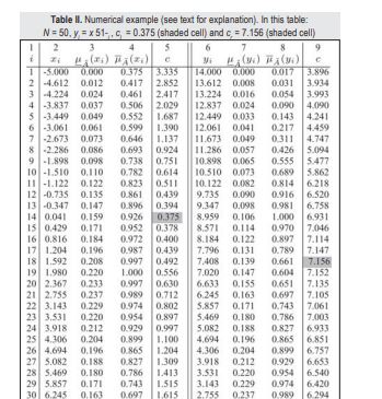
[0.37511, 7.15615]

We can see that this is the Centroid reported by the original authors.

Conclusion

In this post, we have looked at the Centroid of an IT2FS. We have also seen how to use the type2fuzzy library to find such Centroid.