Introduction

In this second part of this series of posts, we will optimize the model we created in the previously by selecting the best set of hyperparameters, or model configuration parameters, that affect the training process. Hyperparameters differ from model parameters in that they are not learnt through some automated process but are chosen by the data scientist. In general, we cannot use techniques to understand model parameters, such as gradient descent, to learn hyperparameters, although they ultimately affect the loss function as well.

The problem of hyperparameter optimization is therefore in finding the optimal model in an $n$ dimensional space; where $n$ is the number of hyperparameters that are being optimized. We refer to this $n$ dimensional space as the search space.

The work described in this section is contained in the following folder structure. In the sections below, we will go through all these files individually.

optimize
│   optimize_model.py
|   requirements.txt
│
└───src
│   │   data_transformer_builder.py
│   │   optimize.py

Hyperparameter Tuning

In AzureML SDK, all modules related to hyperparameter tuning are located in the hyperdrive package. In this section, we will look very briefly at some of the available features. The objective in AzureML hyperparameter tuning is to create a HyperDriveConfig object that defines an optimization run.

Hyperparameters can be discrete or continuous. We can specify continuous hyperparameters over a range of values or a set of values. Discrete hyperparameters are simply a set of values that we can choose and assign a single one to the model. AzureML contains functions to specify discrete and continuous hyperparameter distributions in the parameter_expressions library of the hyperdrive package, where we find the following functions:

• choice() - Specifies a discrete hyperparameter space as a list of possible values.
• lognormal() - Specifies a continuous hyperparameter space as a log-normal distribution with a mean and standard deviation.
• loguniform() - Specifies a continuous hyperparameter space as a log-uniform distribution with a minimum and maximum.
• uniform() - Specifies a continuous hyperparameter space as a uniform distribution with a minimum and maximum.
• normal() - Specifies a continuous hyperparameter space as a normal distribution with a mean and standard deviation.
• quniform() - Specifies a continuous hyperparameter space as a round uniform distribution with a minimum and maximum. quniform() is suitable for discrete hyperparameters.
• qnormal() - Specifies a continuous hyperparameter space as a round-normal distribution with a mean and standard deviation. qnormal() is suitable for discrete hyperparameters.
• randint() - Specifies a discrete hyperparameter space as random integers between zero and a maximum value.

We also require a strategy to navigate the hyperparameter space. The following methods are commonly used in this context are also part of the hyperdrive package:

• RandomParameterSampling. Random sampling selects a random hyperparameter value from the search space. It supports discrete and continuous hyperparameters. Related to the RandomParameterSampling strategy, we can also use the Sobol strategy that covers the search space more evenly.
• GridParameterSampling. Grid sampling supports discrete hyperparameters; however, it is possible to create a discrete set from the distribution of hyperparameters. It goes through the search space defined by choice distributions in a grid fashion.
• BayesianParameterSampling is a more sophisticated strategy that uses a Bayesian approach to select hyperparameters based on the performance of previous hyperparameter selections.

The hyperparameter optimization strategy also requires a primary metric that is being reported in each tuning run. We also need to define the goal for this metric, that is, if our objective is to maximize or minimize it.

Finally, it is also desirable to specify a termination policy that will stop the tuning process when specific parameters are attained.

Model Optimization

This exercise consists of two scripts; the first defines the model optimization strategy, and the second runs the optimization. We will start by looking at the first script.

The first script starts with a definition of the arguments that we will use in the optimization.

'''
Optimization of model parameters
'''
import os
import argparse
import joblib
import pickle
import numpy as np

from sklearn.metrics import mean_squared_error
from sklearn.ensemble import RandomForestRegressor
from sklearn.linear_model import LinearRegression
from sklearn.neighbors import KNeighborsRegressor
from azureml.core import Run, Model, Dataset
import pandas as pd

# Parsing the arguments passed to the script.
parser = argparse.ArgumentParser()
parser.add_argument('--n_estimators', type=int, help='Number of estimators')
parser.add_argument('--base_estimator', type=str, help='Base estimator')
parser.add_argument('--max_samples', type=float, help='Max samples')
parser.add_argument('--max_features', type=float, help='Max features')
parser.add_argument('--bootstrap', type=bool, help='Bootstrap')
args = parser.parse_args()

We then read the train features and labels from the AzureML datasets as numpy arrays.

# get the run context and the workspace.
run = Run.get_context()
workspace = run.experiment.workspace

# Get the dataset for X from the workspace and then mount it.
mount_context_X = Dataset.get_by_name(workspace, name='train_X').mount()
mount_context_X.start()
path = mount_context_X.mount_point + '/data.txt'
train_X = pd.read_csv(path, header=None).to_numpy()
# Get the dataset fot y from the workspace and then mount it.
mount_context_y = Dataset.get_by_name(workspace, name='train_y').mount()
mount_context_y.start()
path = mount_context_y.mount_point + '/data.txt'
train_y = pd.read_csv(path, header=None).to_numpy()

We can then load the data transformer and the machine learning model we previously registered as AzureML models. It is important to note that we need the definition of the custom transformers (the aggregate transformer that was created as part of the train pipeline), and for this reason, we have included the data_transformer_builder.py file.

# Load the data_transformer from the model store.
data_transformer_path = Model(workspace, 'data_transformer').download(exist_ok = True)
data_transformer = joblib.load(data_transformer_path)

# Load the model from the model store.
model_path = Model(workspace, 'concrete_model').download(exist_ok = True)
model = joblib.load(model_path)

At this stage, we can define the machine learning model’s hyperparameters from the arguments passed to the script.

# set the base estimator.
if args.base_estimator == 'LinearRegression':
    model.set_params(base_estimator = LinearRegression())
elif args.base_estimator == 'RandomForestRegressor':
    model.set_params(base_estimator = RandomForestRegressor())
else:
    model.set_params(base_estimator = KNeighborsRegressor())

# Setting the parameters of the model.
model.set_params(n_estimators=args.n_estimators)
# model.set_params(base_estimator=args.base_estimator)
model.set_params(max_samples=args.max_samples)
model.set_params(max_features=args.max_features)
model.set_params(bootstrap=args.bootstrap)

The next step is to obtain the predictions for the train data.

# Transforming the test data using the data transformer and
# then predicting the values using the model.
processed_data = data_transformer.transform(train_X)
predictions = model.predict(processed_data)

Since we have the predictions, we can calculate the RMSE for this set of hyperparameters. We conclude this script by logging the RMSE and storing the model we have created to have a model and metric record for each hyperparameter trial run.

# Calculating square root of the mean squared error.
test_mse = mean_squared_error(train_y, predictions)
sqrt_mse = np.sqrt(test_mse)
run.log('sqrt_mse', sqrt_mse)

# Saving the model to a file.
model_path = os.path.join('outputs', 'model.pkl')
with open(model_path, 'wb') as handle:
    pickle.dump(model, handle, protocol=pickle.HIGHEST_PROTOCOL)

mount_context_X.stop()
mount_context_y.stop()

Execution of Optimization Process

We will now look at how we can execute the optimization process and how to obtain the best model. We start by creating a new ScriptRunConfig object that contains the script’s name that we will execute for each tuning run. we notice that this scripts is executed in the compute target so that we can take advantage of the number of cores available.

'''
Running of experiment_1.py
'''
import os
from azureml.core import Workspace, Experiment, ScriptRunConfig, Environment
from azureml.train.hyperdrive.runconfig import HyperDriveConfig
from azureml.train.hyperdrive.sampling import RandomParameterSampling
from azureml.train.hyperdrive.run import PrimaryMetricGoal, HyperDriveRun
from azureml.train.hyperdrive.parameter_expressions import choice
from azuremlproject import constants

# Loading the workspace from the config file.
config_path = os.path.join(os.path.dirname(os.path.realpath(__file__)), '.azureml')
w_space = Workspace.from_config(path=config_path)

# Creating a ScriptRunConfig object.
config = ScriptRunConfig(
    source_directory=os.path.join(
        os.path.dirname(os.path.realpath(__file__)),
        'src'),
    script='optimize.py',
    compute_target=constants.TARGET_NAME)

We next define the environment that we will use for the experiment. We will attempt to use the same environment we used for the train pipeline, and create it if it does not exist.

if 'concrete_env' in w_space.environments.keys():
    config.run_config.environment = Environment.get(workspace=w_space, name='concrete_env')
else:
    # Creating an environment from the requirements.txt file.
    environment = Environment.from_pip_requirements(
        name='concrete_env',
        file_path=os.path.join(
            os.path.dirname(os.path.realpath(__file__)),
            'requirements.txt')
        )
    config.run_config.environment = environment

We create the hyperparameter search space by instantiating a RandomParameterSampling object that will sample over the hyperparameter search space randomly. The constructor defines the search space as a dictionary of parameter names and ranges. In our case, we are sampling over the following Bagging Regressor hyperparameters:

• n_estimators: Values in the set {5, 10, 15, 20, 25}
• base_estimator: Values in the set {‘LinearRegression’, ‘RandomForestRegressor’, ‘KNeighborsRegressor’}
• max_samples: Values in the set {0.5, 1.0}
• max_features: Values in the set {0.5, 1.0}
• bootstrap: Values in the set [{True, False}

# Creating a dictionary of parameters to be used in the hyperparameter tuning.
param_sampling = RandomParameterSampling( {
    '--base_estimator': choice(
        'LinearRegression', 'RandomForestRegressor', 'KNeighborsRegressor'),
    "--n_estimators": choice(5, 10, 15, 20, 25),
    '--max_samples': choice(0.5, 1.0),
    '--max_features': choice(0.5, 1.0),
    '--bootstrap': choice(1, 0),
    }
)

We can then create a HyperDriveConfig object that we will use to execute the optimization process. The constructor defines several parameters, including:

• The instance of the RunConfig object will be used to execute the script.
• The instance of the ParameterSampling object that will be used to sample over the hyperparameter search space.
• The Primary Metric Name or the parameter that will be used to compare the various hyperparameter trials.
• The Primary Metric Goal defines our objective with the metric, maximization or minimization.
• The Maximum Number of Trials that will be used to execute the optimization process. The trial will terminate when this number of trials is reached.
• The Number of concurrent trials will be used to execute the optimization process. This number depends on the AzureML compute we selected to run the experiment.

# Creating a hyperdrive configuration object.
hyperdrive_config = HyperDriveConfig(run_config=config,
                                    hyperparameter_sampling=param_sampling,
                                    primary_metric_name='sqrt_mse',
                                    primary_metric_goal=PrimaryMetricGoal.MINIMIZE,
                                    max_total_runs=4,
                                    max_concurrent_runs=4)

We can then submit the experiment to the workspace for execution. We have used the name concrete_tune as the experiment’s name.

# This is submitting the hyperdrive configuration to the experiment.
experiment = Experiment(w_space, 'concrete_tune')
run:HyperDriveRun = experiment.submit(hyperdrive_config )
run.wait_for_completion(show_output=True)

We assert that the experiment has been completed successfully.

# Checking if the run is completed.
assert run.get_status() == "Completed"
# Printing the status of the run.
print('status', run.get_status())

We can then get the best model from the experiment. In this case, we are printing the RMSE and the values of the hyperparameters of the best run. We then register the best model to the workspace with the name final_model.

best_run = run.get_best_run_by_primary_metric()
print('best_run', best_run)
best_run_metrics = best_run.get_metrics()
print('best_run_metrics', best_run_metrics)
parameter_values = best_run.get_details()['runDefinition']['arguments']
print('parameter_values', parameter_values)
best_run.register_model(model_name='final_model', model_path="outputs/model.pkl")

Execution

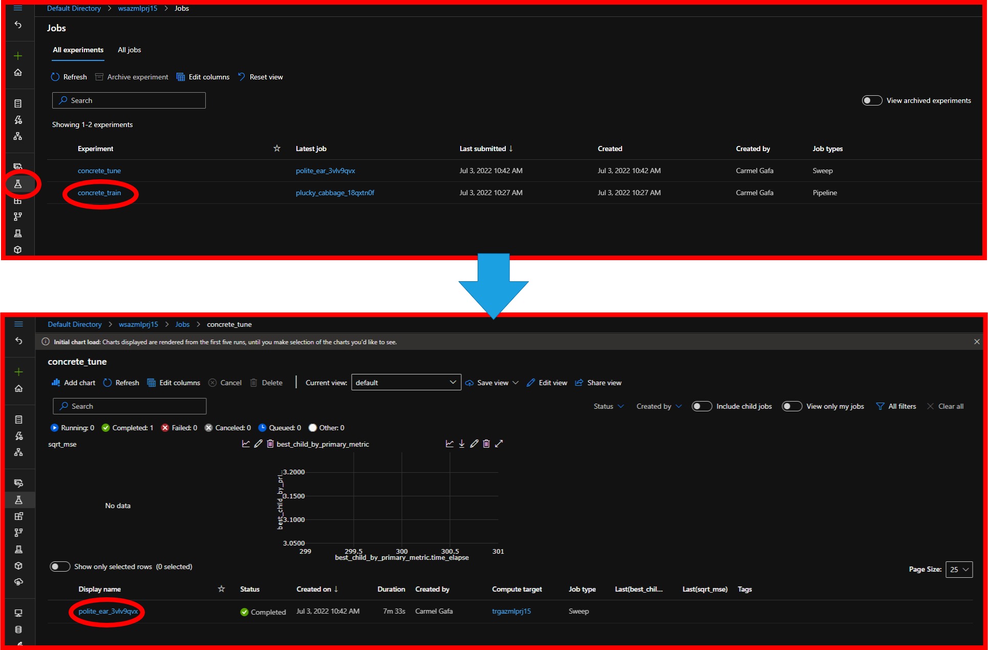
Navigating the workspace experiments, we notice a new experiment called concrete_tune. The experiment will contain all the runs that we executed for this experiment.

Each run will contain information about the execution organized in some tabs:

• Metrics: This tab contains the metrics calculated during the run.
• Overview: This tab contains a summary of the run.
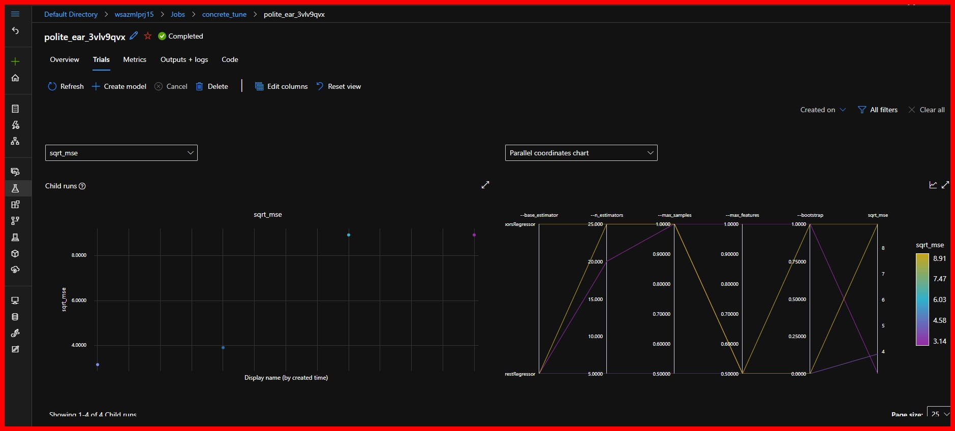
• Trials: This tab contains the trials (different hyperparameter combinations) we executed during the run.
• Output+Logs: This tab contains the output and logs files of the run.

Overview of the run. Observe the search space definition

The trials tab provides valuable information about the run. The parallel coordinates chart shows the various hyperparameter combination effect on the cost function

Now, we can see the workspace models; we can see that the best model has been registered to the workspace with the name final_model.

The final model

The run execution also leaves some interesting information in our console, including the hyperparameters that we used to train the best model.

References

[1] Microsoft, Hyperparameter tuning a model (v2) - Azure Machine Learning [online] [Accessed 20 June 2022]

[2] Microsoft azureml.train.hyperdrive package [online] [Accessed 1 July 2022].

[3] Brownlee, J., Machine Learning Mastery - Hyperparameter Optimization With Random Search and Grid Search [online] [Accessed 2 July 2022]